Hypothesis tests

Author

Affiliation

Beniamino Sartini

University of Bologna

library(dplyr)
library(ggplot2)
# ================== Setups ==================
n <- 500 # number of simulations 
set.seed(1) # random seed 
mu_0 <- 2.4 # H0 mean 
mu_true <- 2 # true mean
alpha <- 0.05 # confidence level
# ============================================
# Simulated random variable 
Xn <- rnorm(n, mean = mu_true, sd = 4)
# Grid of points for pdf
x <- seq(-4, 4, 0.01)
x_breaks <- seq(min(x), max(x), 1)

A statistical hypothesis test is a method of statistical inference used to decide whether the data sufficiently support a particular hypothesis. An hypothesis test typically involves a calculation of a test statistic, that under the null hypothesis \(H_0\) can assume a certain distribution. Then a decision is made, either by comparing the test statistic to a critical value or equivalently by evaluating a p-value computed from the test statistic. Then, the purpose of a test is to reject or not the null hypothesis at a fixed a confidence level \(\alpha\). Note that an hypothesis is never accepted, but always non-rejected. In general, two kind of tests are available:

• A two-tailed test is appropriate if the estimated value is greater or less than a certain range of values, for example, whether a test taker may score above or below a specific range of scores.

• A one-tailed test is appropriate if the estimated value may depart from the reference value in only one direction, left or right, but not both.

Let’s consider a \(t-test\) for the mean of a sample \(X_n = (x_1, \dots, x_i, \dots, x_n)\), i.e.  \[ T(X_n) = \frac{\mu(X_n) - \mu_{0}}{\frac{\sigma(X_n)}{\sqrt{n}}} \overset{H_0}{\sim} t_{n-1} \underset{n\to \infty}{\longrightarrow} \mathcal{N}(0,1) \] where \(\mu(X)\) is the sample mean, \(\sigma(X)\) is an unbiased estimator of the population standard deviation and \(\mu_0\) is the mean under the null hypothesis \(H_0\). The statistic test under \(H_0\) follows a student-t distribution with \(n-1\) degrees of freedom. Notably, for large samples the statistic converges to a normal random variable.

1 Two-tail test

For example, let’s simulate a sample \(X_n\) of \(n = 500\) observations from a normal distribution (i.e. \(X_n \sim \mathcal{N}(2, 4^2)\)). Then, let’s consider the hypothesis: \[ H_0: \mu(X) = 2.4 \quad\quad H_1: \mu(X) \neq 2.4 \] and the statistic test is then defined as: \[ T(X_n) = \sqrt{500}\frac{\mu(X_n) - 2.4}{\sigma(X_n)} \overset{H_0}{\sim} t(499) \text{.} \]

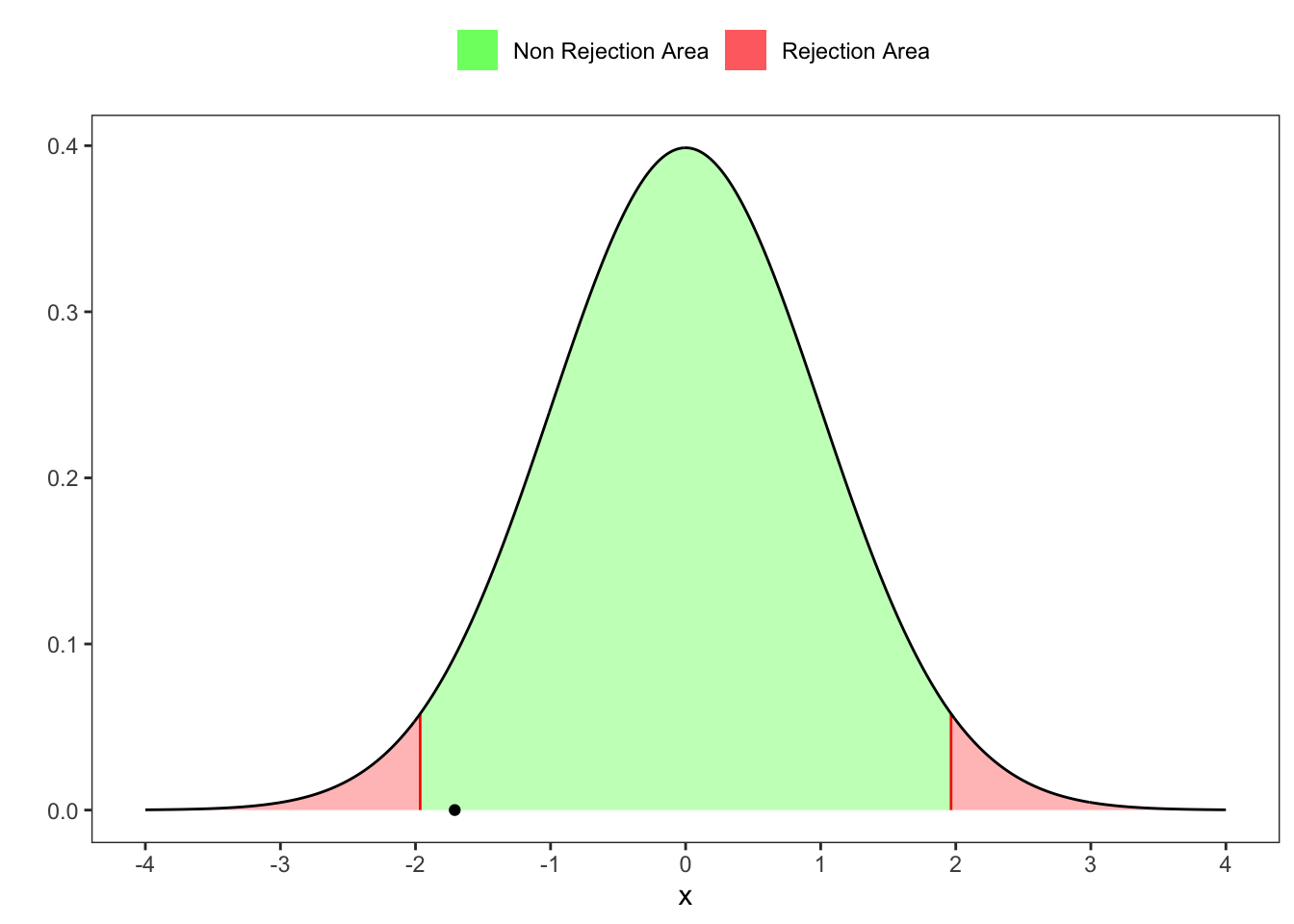
Since it is a two-tailed test the critical value at a confidence level \(\alpha\), denoted as \(t_{\alpha}\), is such that: \[ \begin{align} \alpha & = \mathbb{P}([T(X_n) < -t_{\alpha/2}] \cup [T(X_n) > t_{\alpha/2}]) \\ \Updownarrow & \\ t_{\alpha/2} & = \mathbb{P}^{-1}(\mathbb{P}(T(X_n) > t_{\alpha/2})) \text{,} \end{align} \] where \(\mathbb{P}^{-1}\) and \(\mathbb{P}\) are respectively the quantile and distribution functions of a Student-\(t\). Hence, with \(\alpha = 0.05\) if \(-1.9604 < T(X_n) < 1.9604\) we do not reject the null hypothesis, i.e. \(\mu(X_n)\) is equal to \(\mu_{0} = 2.4\), otherwise we reject it, i.e. the two means are different.

# Statistic T
z <- sqrt(n)*(mean(Xn) - mu_0)/sd(Xn)
pdf <- dt(x, df = n-1)
# Critical value left 
z_left <- c(qt(alpha/2, df = n-1), dt(qt(alpha/2, df = n-1), df = n-1))
# Critical value right 
z_right <- c(qt(1-alpha/2, df = n-1), dt(qt(1-alpha/2, df = n-1), df = n-1))
ggplot()+
  geom_segment(aes(x = z_left[1], xend = z_left[1], y = 0, yend = z_left[2]), color = "red")+
  geom_segment(aes(x = z_right[1], xend = z_right[1], y = 0, yend = z_right[2]), color = "red")+
  geom_ribbon(aes(x = x[x < z_left[1]], ymin = 0, ymax = dt(x[x < z_left[1]], df = n-1), fill = "rej"), alpha = 0.3)+
  geom_ribbon(aes(x = x[x > z_right[1]], ymin = 0, ymax = dt(x[x > z_right[1]], df = n-1), fill = "rej"), alpha = 0.3)+
  geom_ribbon(aes(x = x[x > z_left[1] & x < z_right[1]], ymin = 0, ymax = dt(x[x > z_left[1] & x < z_right[1]], df = n-1), 
                  fill = "norej"), alpha = 0.3)+
  geom_line(aes(x, pdf))+
  geom_point(aes(z, 0), color = "black")+
  scale_fill_manual(values = c(rej = "red", norej = "green"), 
                    labels = c(rej = "Rejection Area", norej = "Non Rejection Area")) + 
  scale_x_continuous(breaks = x_breaks) +
  labs(y = "", x = "x", fill = NULL)+
  theme_bw()+
  theme(
    legend.position = "top",
    panel.grid = element_blank()
  )

Figure 1: Two-tailed test on the mean.

2 Left-tailed test

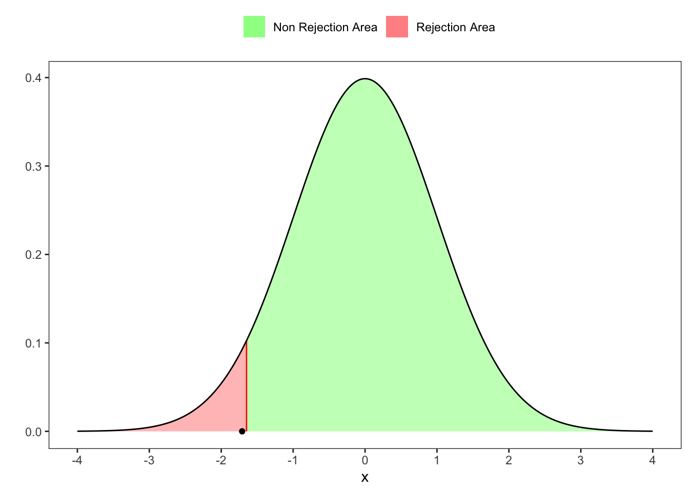
For example, let’s consider another the hypothesis: \[ H_0: \mu(X) \ge 2.4 \quad\quad H_1: \mu(X) < 2.4 \] The statistic test \(T(X_n)\) do not changes, however it is a left-tailed test. Hence, the critical value is \(t_{\alpha}\) is such that \(\mathbb{P}(x < t_{\alpha}) = 0.05\). Applying the quantile function \(\mathbb{P}^{-1}\) of a student-\(t\) we obtain: \[ \begin{align} \alpha & = \mathbb{P}(T(X_n) < t_{\alpha}) \\ \Updownarrow & \\ t_{\alpha} & = \mathbb{P}^{-1}(\mathbb{P}(T(X_n) < t_{\alpha})) \text{,} \end{align} \] where \(\mathbb{P}^{-1}\) and \(\mathbb{P}\) are respectively the quantile and distribution functions of a Student-\(t\). Hence, for \(\alpha = 0.05\) if \(T(X_n) < -1.6451\) we do not reject the null hypothesis, i.e. \(\mu(X_n)\) is greater than \(\mu_{0}\), otherwise we reject it and \(\mu(X_n)\) is lower than \(\mu_{0}\).

# Critical value left 
z_left <- c(qt(alpha, df = n-1), dt(qt(alpha, df = n-1), df = n-1))
ggplot()+
  geom_segment(aes(x = z_left[1], xend = z_left[1], y = 0, yend = z_left[2]), color = "red")+
  geom_ribbon(aes(x = x[x < z_left[1]], ymin = 0, ymax = dt(x[x < z_left[1]], df = n-1), fill = "rej"), alpha = 0.3)+
  geom_ribbon(aes(x = x[x > z_left[1]], ymin = 0, ymax = dt(x[x > z_left[1]], df = n-1), 
                  fill = "norej"), alpha = 0.3)+
  geom_line(aes(x, pdf))+
  geom_point(aes(z, 0), color = "black")+
  scale_fill_manual(values = c(rej = "red", norej = "green"), 
                    labels = c(rej = "Rejection Area", norej = "Non Rejection Area")) + 
  scale_x_continuous(breaks = x_breaks) +
  labs(y = "", x = "x", fill = NULL)+
  theme_bw()+
  theme(
    legend.position = "top",
    panel.grid = element_blank()
  )

Figure 2: Left-tailed test on the mean.

In this case we reject the null hyphotesis, hence \(\mu(X_n)\) is lower than \(\mu_{0}\).

3 Right-tailed test

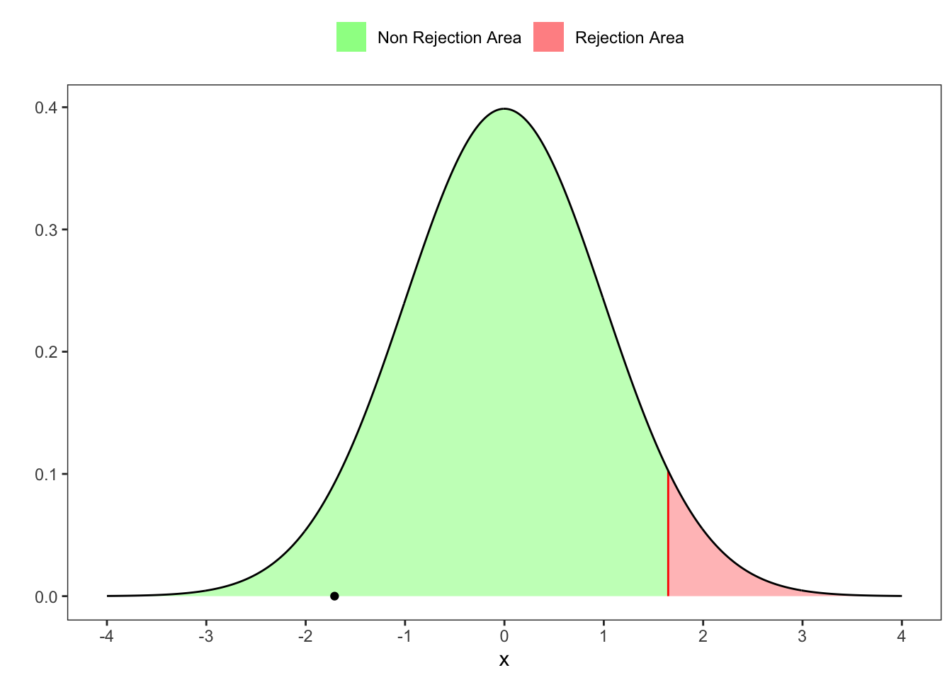
Let’s consider the other case, i.e. \[ H_0: \mu(X) \le 2.4 \quad\quad H_1: \mu(X) > 2.4 \] It is always one-side test, but in this case is right-tailed. Hence, the critical value \(t_{\alpha}\) is such that \[ \begin{align} 1-&\alpha = \mathbb{P}(T(X_n) < t_{\alpha}) \\ \Updownarrow & \\ t_{\alpha} & = \mathbb{P}^{-1}(\mathbb{P}(T(X_n) < t_{\alpha})) \text{,} \end{align} \] where \(\mathbb{P}^{-1}\) and \(\mathbb{P}\) are respectively the quantile and distribution functions of a Student-\(t\). Hence, for \(\alpha = 0.05\) if \(T(X_n) > 1.6451\) we do not reject the null hypothesis, i.e. \(\mu(X_n)\) is lower than \(\mu_{0}\), otherwise we reject it and \(\mu(X_n)\) is greater than \(\mu_{0}\).

# Critical value right 
z_right <- c(qt(1-alpha, df = n-1), dt(qt(1-alpha, df = n-1), df = n-1))
ggplot()+
  geom_segment(aes(x = z_right[1], xend = z_right[1], y = 0, yend = z_right[2]), color = "red")+
  geom_ribbon(aes(x = x[x > z_right[1]], ymin = 0, ymax = dt(x[x > z_right[1]], df = n-1), fill = "rej"), alpha = 0.3)+
  geom_ribbon(aes(x = x[x < z_right[1]], ymin = 0, ymax = dt(x[x < z_right[1]], df = n-1), 
                  fill = "norej"), alpha = 0.3)+
  geom_line(aes(x, pdf))+
  geom_point(aes(z, 0), color = "black")+
  scale_fill_manual(values = c(rej = "red", norej = "green"), 
                    labels = c(rej = "Rejection Area", norej = "Non Rejection Area")) + 
  scale_x_continuous(breaks = x_breaks) +
  labs(y = "", x = "x", fill = NULL)+
  theme_bw()+
  theme(
    legend.position = "top",
    panel.grid = element_blank()
  )

Figure 3: Right-tailed test on the mean.

Coherently with the previous test in this case we don’t reject \(H_0\), hence \(\mu(X_n)\) is lower than \(\mu_{0} = 2.4\).