Normality tests

Author

Affiliation

Beniamino Sartini

University of Bologna

library(dplyr) 
library(ggplot2)
library(knitr)

Tests of normality are statistical inference procedures designed to test that the underlying distribution of a random variable is normally distributed. There is a long history of these tests, and there are a plethora of them available for use, i.e. Jarque and Bera (1980), D’Agostino and Pearson (1973), Ralph B. D’agostino and Jr. (1990). Such kind of tests are based on the comparison of the sample skewness and kurtosis with the skewness and kurtosis of a normal distribution, hence their estimation is crucial.

1 Theoric Moments

1.1 Expectation

Let’s define and denote the expectation in population of a random variable \(X\) as \[ \mathbb{E}\{X\} = \mu(X) \] whereas the sample’s expectation on \(X_n = (x_1, \dots, x_i, \dots, x_n)\) is denoted as: \[ \mathbb{E}\{X_n\} = \hat{\mu}(X_n) = \frac{1}{n}\sum_{i = 1}^{n}x_i \]

1.2 Variance

Let’s define and denote the population variance of a random variable \(X\) as: \[ \mathbb{V}\{X\} = \sigma(X) = \mathbb{E}\{\left(X - \mathbb{E}\{X\}\right)^2\} \text{,} \] whereas the sample’s variance on \(X_n = (x_1, \dots, x_i, \dots, x_n)\) is denoted as: \[ \mathbb{V}\{X_n\} = \hat{\sigma}^2(X_n) = \frac{1}{n}\sum_{i = 1}^{n} \left(x_i - \mathbb{E}\{X_n\}\right)^2 \text{.} \] To correct the estimator \(\hat{\sigma}^2(X_n)\) let’s define: \[ \hat{s}^2(X_n) = \frac{1}{n-1}\sum_{i = 1}^{n} \left(x_i - \mathbb{E}\{X_n\}\right)^2 \text{,} \] where \(\hat{s}^2(X_n) = \frac{n}{n-1}\hat{\sigma}^2(X_n)\).

1.3 Skewness

Following the same notation as in Ralph B. D’agostino and Jr. (1990), let’s define and denote the population skewness of a random variable \(X\) as: \[ \mathbb{S}k\{X\} = \beta_1(X) = \mathbb{E}\left\{\left(\frac{X - \mathbb{E}\{X\}}{\sqrt{\mathbb{V}\{X\}}}\right)^3\right\} \text{,} \] whereas the sample’s skewness on \(X_n = (x_1, \dots, x_i, \dots, x_n)\) is denoted as: \[ \mathbb{S}k\{X_n\} = b_1(X_n) = \frac{1}{n}\sum_{i = 1}^{n} \left(\frac{x_i - \mathbb{E}\{X_n\}}{\sqrt{\mathbb{V}\{X_n\}}}\right)^3 \text{.} \tag{1}\] To correct the estimator \(b_1(X_n)\) let’s define: \[ g_1(X_n) = \frac{\sqrt{n(n-1)}}{(n-2)} b_1(X_n) \text{.} \] Notably the asymptotic distribution of the sample skewness is normal, i.e. \[ b_1(X_n) \underset{n \to \infty}{\overset{d}{\longrightarrow}} \mathcal{N}\left(0, \frac{6}{n} \right) \text{.} \tag{2}\]

Notably, in Urzúa (1996) are reported also the exact mean of the estimator in Equation 1 when \(X \sim \mathcal{N}\), i.e.
\[ \mathbb{E}\{b_1(X_n)\} = 0 \text{,} \] and the variance \[ \mathbb{V}\{b_1(X_n)\} = \frac{6(n-2)}{(n+1)(n+3)} \text{.} \tag{3}\]

skewness <- function(x, na.rm = FALSE){
  e_x <- mean(x, na.rm = na.rm)
  sd_x <- sd(x, na.rm = na.rm)
  mean((x - e_x)^3, na.rm = na.rm)/(sd_x^3)
}

1.4 Kurtosis

Let’s define and denote the population kurtosis of a random variable \(X\) as: \[ \mathbb{K}t\{X\} = \beta_2(X) = \mathbb{E}\left\{\left(\frac{X - \mathbb{E}\{X\}}{\sqrt{\mathbb{V}\{X\}}}\right)^4\right\} \text{,} \] whereas the sample’s kurtosis on \(X_n = (x_1, \dots, x_i, \dots, x_n)\) is denoted as: \[ \mathbb{K}t\{X_n\} = b_2(X_n) = \frac{1}{n}\sum_{i = 1}^{n} \left(\frac{x_i - \mathbb{E}\{X_n\}}{\sqrt{\mathbb{V}\{X_n\}}}\right)^4 \text{.} \tag{4}\] From Pearson (1931), we have a correct the version of \(b_1(X_n)\) defined as: \[ g_2(X_n) = \left[b_2(X_n) - \frac{3(n+1)}{n+1} \right]\frac{(n+1)(n-1)}{(n-2)(n-3)} \text{.} \] The asymptotic distribution of the sample kurtosis is normal, i.e. \[ b_2(X_n) \underset{n \to \infty}{\overset{d}{\longrightarrow}} \mathcal{N}\left(3, \frac{24}{n} \right) \text{.} \tag{5}\]

Notably in Urzúa (1996) are reported also the exact mean when \(X \sim \mathcal{N}\) \[ \mathbb{E}\{b_2(X_n)\} = \frac{3(n-1)}{(n+1)} \text{,} \tag{6}\]

and the variance as: \[ \mathbb{V}\{b_2(X_n)\} = \frac{24n(n-2)(n-3)}{(n+1)^2(n+3)(n+5)} \text{.} \tag{7}\]

kurtosis <- function(x, na.rm = FALSE, excess = TRUE){
  e_x <- mean(x, na.rm = na.rm)
  sd_x <- sd(x, na.rm = na.rm)
  mean((x - e_x)^4, na.rm = na.rm)/(sd_x^4) - ifelse(excess, 3, 0)
}

2 Jarque-Brera test

If \(X\) is an independent and identically distributed process, the asymptotic distribution of the skewness and kurtosis in Equation 2 holds for \(X \sim \mathcal{N}\). Hence, we construct an omnibus test for normality. Standardizing the skewness and kurtosis, under \[ H_0: \beta_1(X_n) = 0, \, \beta_2(X_n) = 3 \text{,} \] we have
\[ \begin{aligned} {} & Z_1(X_n) = \sqrt{n} \frac{b_1(X_n)}{\sqrt{6}} \underset{n \to \infty}{\overset{d}{\longrightarrow}} \mathcal{N}\left(0, 1\right) \text{,} \\ & Z_2(X_n) = \sqrt{n} \frac{b_2(X_n)-3}{\sqrt{24}}\underset{n \to \infty}{\overset{d}{\longrightarrow}} \mathcal{N}\left(0, 1\right) \text{,} \end{aligned} \] where \(b_1(X_n)\) and \(b_2(X_n)\) are defined respectively in Equation 1 and in Equation 4. It is possible to prove that \(Z_1(X_n)\) and \(Z_2(X_n)\) are independent. Since the sum of two independent standard normal squared random variables follows a \(\chi^{2}_{v}\) distribution with \(v = 2\) degrees of freedom, let’s rewrite the Jarque-Brera statistic as: \[ \text{JB}(X_n) = Z_1(X_n)^2 + Z_2(X_n)^2 \underset{n \to \infty}{\overset{d}{\longrightarrow}} \chi^{2}_{2} \text{.} \] However, if \(n\) is small the \(\text{JB}(X_n)\) over-reject the null hypothesis \(H_0\), i.e. type I error.

# =============== Setups =============== 
n <- 50 # number of simulations 
set.seed(1) # random seed 
ci <- 0.05 # confidence level 
# ======================================
# Simulated variable 
x <- rnorm(n, 0, 1)
# Sample skewness
b1 <- skewness(x)
# Sample kurtosis 
b2 <- kurtosis(x, excess = F)
# JB-statistic test
JB <- n*(b1^2/6 + (b2 - 3)^2/24)
# JB-test pvalue 
pvalue <-  1 - pchisq(JB, df = 2)
# JB-test critic value at 95%
z_lim <- qchisq(1-ci, 2)
# =============== Plot =============== 
# Grid of points 
grid <- seq(0, 10, 0.01)
# Rejection area 
grid_rej <- grid[grid > z_lim]
# Non-rejection area 
grid_norej <- grid[grid < z_lim]
ggplot()+
  geom_line(aes(grid, dchisq(grid, 2)))+
  geom_segment(aes(z_lim, xend = z_lim, y = 0, yend = dchisq(z_lim, 2)))+
  geom_point(aes(JB, 0))+
  geom_ribbon(aes(x = grid_rej, ymin = 0, ymax = dchisq(grid_rej, 2), fill = "rej"), alpha = 0.3)+
  geom_ribbon(aes(x = grid_norej, ymin = 0, ymax = dchisq(grid_norej, 2), fill = "norej"), alpha = 0.3)+
  geom_segment(aes(JB, xend = JB, y = 0, yend = dchisq(JB, 2)))+
  scale_x_continuous(breaks = c(0, JB, z_lim), 
                     labels = c("0", format(c(JB, z_lim), digits = 4)))+
  labs(x = "JB statistic", y = "", fill = NULL)+
  scale_fill_manual(values = c(rej = "red", norej = "green"), 
                    labels = c(rej = "Rejection Area", norej = "Non Rejection Area")) + 
  theme_bw()+
  theme(
    legend.position = "top",
    panel.grid = element_blank()
  )

Figure 1: Jarque-Brera test for normality with a simulated Normal sample of 50 observations with \(\alpha = 0.05\).

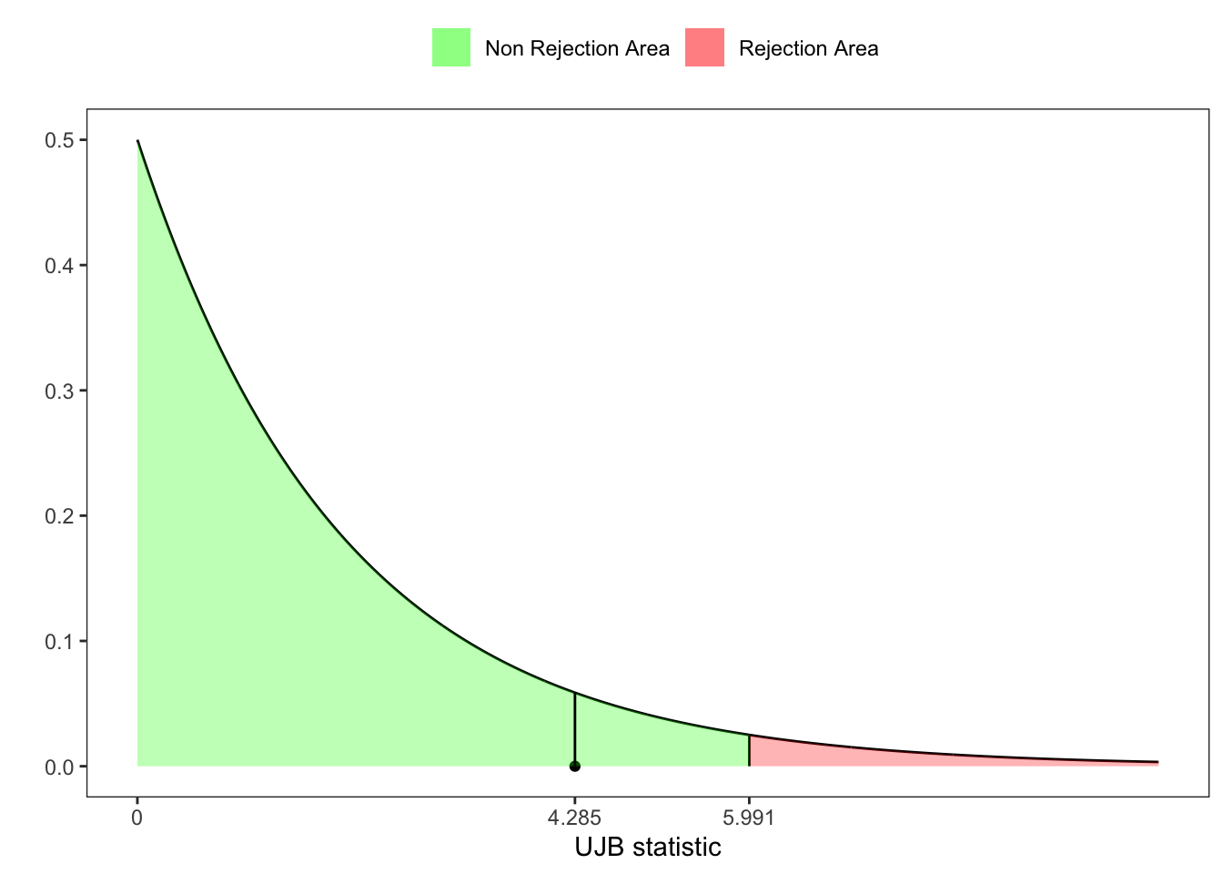
3 Urzua-Jarque-Brera test

Let’s substitute the asymptotic moments with the exact sample moments of skewness and kurtosis. Following Urzúa (1996), let’s write the new omibus test statistic as: \[ \begin{aligned} {} & \tilde{Z}_1(X_n) = \frac{b_1(X_n)}{\sqrt{\mathbb{V}\{b_1(X_n)\}}} \underset{n \to \infty}{\overset{d}{\longrightarrow}} \mathcal{N}\left(0, 1\right) \text{,} \\ & \tilde{Z}_2(X_n) = \frac{b_2(X_n) - \mathbb{E}\{b_2(X_n)\}}{\sqrt{\mathbb{V}\{b_2(X_n)\}}} \underset{n \to \infty}{\overset{d}{\longrightarrow}} \mathcal{N}\left(0, 1\right) \text{,} \end{aligned} \] where the exact moments \(\mathbb{V}\{b_1(X_n)\}\), \(\mathbb{E}\{b_2(X_n)\}\) and \(\mathbb{V}\{b_2(X_n)\}\) are defined respectively in Equation 3, Equation 6, Equation 7. Hence, the Urzua-Jarque-Brera test adjusted for small samples is computed as: \[ \text{UJB}(X_n) = \tilde{Z}_1(X_n)^2 + \tilde{Z}_2(X_n)^2 \underset{n \to \infty}{\overset{d}{\longrightarrow}} \chi^{2}_{2} \text{.} \]

# =============== Setups =============== 
n <- 50 # number of simulations 
set.seed(1) # random seed 
ci <- 0.05 # confidence level 
# ======================================
# Simulated variable 
x <- rnorm(n, 0, 1)
# Sample skewness
b1 <- skewness(x)
# Skewness's variance
v_b1 <- (6*(n-2))/((n+1)*(n+3))
# Statistic for skewness
Z1 <- b1/sqrt(v_b1)
# Sample kurtosis 
b2 <- kurtosis(x, excess = F)
# Kurtosis's expected value
e_b2 <- (3*(n-1))/(n+1)
# Kurtosis's variance
v_b2 <- (24*n*(n-2)*(n-3))/((n+1)^2*(n+3)*(n+5))
# Statistic for kurtosis
Z2 <- (b2-e_b2)/sqrt(v_b2)
# UJB-statistic test
UJB <- Z1^2 + Z2^2
# UJB p-value 
pvalue <-  1 - pchisq(UJB, df = 2)
# UJB critic value at 95%
z_lim <- qchisq(1-ci, 2)
# =============== Plot =============== 
# Grid of points 
grid <- seq(0, 10, 0.01)
# Rejection area 
grid_rej <- grid[grid > z_lim]
# Non-rejection area 
grid_norej <- grid[grid < z_lim]
ggplot()+
  geom_line(aes(grid, dchisq(grid, 2)))+
  geom_segment(aes(z_lim, xend = z_lim, y = 0, yend = dchisq(z_lim, 2)))+
  geom_point(aes(UJB, 0))+
  geom_ribbon(aes(x = grid_rej, ymin = 0, ymax = dchisq(grid_rej, 2), fill = "rej"), alpha = 0.3)+
  geom_ribbon(aes(x = grid_norej, ymin = 0, ymax = dchisq(grid_norej, 2), fill = "norej"), alpha = 0.3)+
  geom_segment(aes(UJB, xend = UJB, y = 0, yend = dchisq(UJB, 2)))+
  scale_x_continuous(breaks = c(0, UJB, z_lim), 
                     labels = c("0", format(c(UJB, z_lim), digits = 4)))+
  labs(x = "UJB statistic", y = "", fill = NULL)+
  scale_fill_manual(values = c(rej = "red", norej = "green"), 
                    labels = c(rej = "Rejection Area", norej = "Non Rejection Area")) + 
  theme_bw()+
  theme(
    legend.position = "top",
    panel.grid = element_blank()
  )

Figure 2: Urzua-Jarque-Brera test for normality with a simulated Normal sample of 50 observations with \(\alpha = 0.05\).

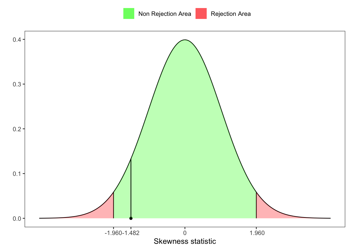
4 D’Agostino skewness test

D’Agostino and Pearson (1973) proposed an alternative way to test that the skewness is different from zero. Starting from the statistic \(\tilde{Z}_1(X_n)\), compute: \[ \beta_2(b_1) = \frac{3 (n^2 + 27n -70)(n+1)(n+3)}{(n-2)(n+5)(n+7)(n+9)} \text{,} \] and \[ \begin{aligned} {} & W^2 = \sqrt{2 \beta_2(b_1) - 1 } -1 \text{,} \\ & \delta = \frac{1}{\sqrt{\ln(W)}} \text{,} \\ & \alpha = \sqrt{\frac{2}{W^2 - 1}} \text{.} \end{aligned} \] The statistic test for skewness is defined as:
\[ \begin{aligned}Z_1^{\ast}(X_n) {} & = \delta \log \left\{\frac{\tilde{Z}_1(X_n)}{\alpha} + \sqrt{\left(\frac{\tilde{Z}_1(X_n)}{\alpha}\right)^2 + 1}\right\} = \\ & = \delta \sinh^{-1}\left( \frac{\tilde{Z}_1(X_n)}{\alpha}\right)\text{,}\end{aligned} \] where \(Z_1^{\ast}(X_n) \sim \mathcal{N}(0,1)\).

# =============== Setups =============== 
n <- 20 # number of simulations 
set.seed(1) # random seed 
ci <- 0.05 # confidence level 
# ======================================
# Simulated variable 
x <- rnorm(n, 0, 1)
# Sample skewness
b1 <- skewness(x)
# Skewness's variance
v_b1 <- (6*(n-2))/((n+1)*(n+3))
# Statistic for skewness
Z1 <- b1/sqrt(v_b1)
# Test for Skewness 
beta2_b1 <- (3*(n^2 + 27*n - 70)*(n+1)*(n+3))/((n-2)*(n+5)*(n+7)*(n+9))
W2 <- sqrt(2*beta2_b1 - 1) - 1
delta <- 1/sqrt(log(sqrt(W2)))
alpha <- sqrt(2/(W2 - 1))
# Test for skewness
Z_ast_b1 <- delta*asinh(Z1/alpha)
# UJB p-value 
pvalue <- 1 - pnorm(Z_ast_b1, lower.tail = TRUE)
# UJB critic value at 95%
z_lim <- qnorm(1-ci/2)
# =============== Plot =============== 
# Grid of points 
grid <- seq(-4, 4, 0.01)
# Rejection area 
grid_rej_l <- grid[grid >= z_lim]
grid_rej_r <- grid[grid <= -z_lim]
# Non-rejection area 
grid_norej <- grid[!(grid > z_lim | grid < -z_lim)]
ggplot()+
  geom_line(aes(grid, dnorm(grid)))+
  geom_segment(aes(z_lim, xend = z_lim, y = 0, yend = dnorm(z_lim)))+
  geom_segment(aes(-z_lim, xend = -z_lim, y = 0, yend = dnorm(-z_lim)))+
  geom_point(aes(Z_ast_b1, 0))+
  geom_ribbon(aes(x = grid_rej_l, ymin = 0, ymax = dnorm(grid_rej_l), fill = "rej"), alpha = 0.3)+
  geom_ribbon(aes(x = grid_rej_r, ymin = 0, ymax = dnorm(grid_rej_r), fill = "rej"), alpha = 0.3)+
  geom_ribbon(aes(x = grid_norej, ymin = 0, ymax = dnorm(grid_norej), fill = "norej"), alpha = 0.3)+
  geom_segment(aes(Z_ast_b1, xend = Z_ast_b1, y = 0, yend = dnorm(Z_ast_b1)))+
  scale_x_continuous(breaks = c(0, Z_ast_b1, z_lim, -z_lim), 
                     labels = c("0", format(c(Z_ast_b1, z_lim, -z_lim), digits = 4)))+
  labs(x = "Skewness statistic", y = "", fill = NULL)+
  scale_fill_manual(values = c(rej = "red", norej = "green"), 
                    labels = c(rej = "Rejection Area", norej = "Non Rejection Area")) + 
  theme_bw()+
  theme(
    legend.position = "top",
    panel.grid = element_blank()
  )

Figure 3: Skewness test with a simulated Normal sample of 50 observations with \(\alpha = 0.05\).

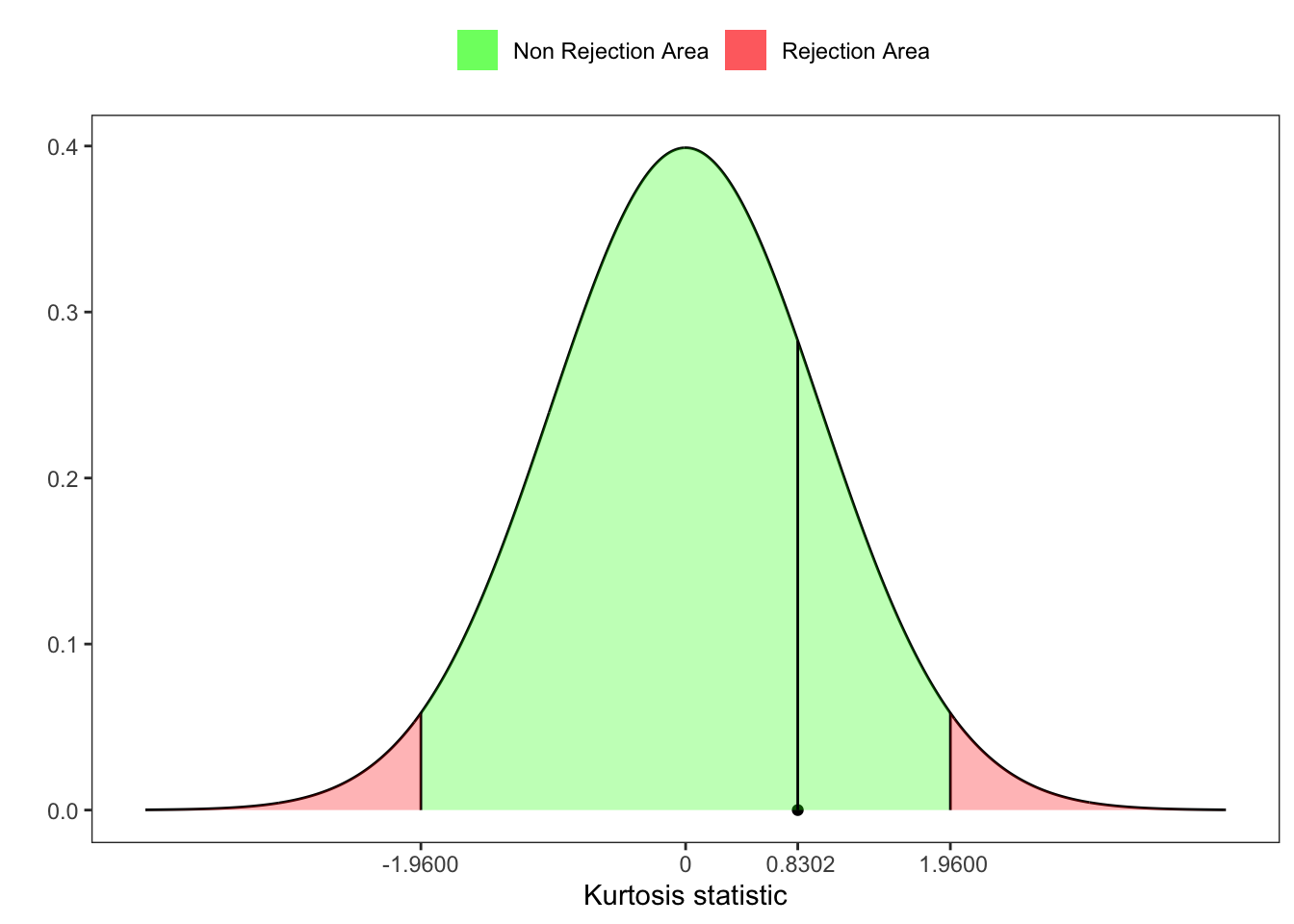
5 Anscombe Kurtosis test

Anscombe and Glynn (1983) proposed a test for skewness. Starting from the statistic \(\tilde{Z}_2(X_n)\), let’s compute the third standardized moment of \(b_2\): \[ \beta_1(b_2) = \frac{6(n^2 - 5n + 2)}{(n+7)(n+9)}\sqrt{\frac{6(n+3)(n+5)}{n(n-2)(n-3)}} \text{,} \] and \[ A = 6 + \frac{8}{\beta_1(b_2)} \left[\frac{2}{\beta_1(b_2)} + \sqrt{1 + \frac{4}{\beta_1(b_2)}}\right] \text{.} \] The statistic test for kurtosis is defined as: \[ Z_2^{\ast}(X_n) = \sqrt{\frac{9A}{2}}\left(1 - \frac{2}{9A} - \left[\frac{1 - 2/A}{1 + \tilde{Z}_2(X_n) \sqrt{2/(A - 4)} } \right]^{1/3} \right) \text{,} \] where \(Z_2^{\ast}(X_n) \sim \mathcal{N}(0,1)\).

# =============== Setups =============== 
n <- 50 # number of simulations 
set.seed(1) # random seed 
ci <- 0.05 # confidence level 
# ======================================
# Simulated variable 
x <- rnorm(n, 0, 1)
# Sample kurtosis 
b2 <- kurtosis(x, excess = F)
# Kurtosis's expected value
e_b2 <- (3*(n-1))/(n+1)
# Kurtosis's variance
v_b2 <- (24*n*(n-2)*(n-3))/((n+1)^2*(n+3)*(n+5))
# Statistic for kurtosis
Z2 <- (b2-e_b2)/sqrt(v_b2)
# Test for Skewness 
beta1_b2 <- (6*(n^2 - 5*n + 2))/((n+7)*(n+9))*sqrt((6*(n+3)*(n+5))/(n*(n-2)*(n-3)))
A <- 6 + (8/beta1_b2)*(2/beta1_b2 + sqrt(1 + 4/(beta1_b2^2)))
# Test for kurtosis
Z_ast_b2 <- sqrt((9*A)/2) *(1 - 2/(9*A) - ((1 - 2/A)/(1 + Z2*sqrt(2/(A-4))))^(1/3))
# p-value 
pvalue <- 1 - pnorm(Z_ast_b2, lower.tail = TRUE)
# UJB critic value at 95%
z_lim <- qnorm(1-ci/2)
# =============== Plot =============== 
# Grid of points 
grid <- seq(-4, 4, 0.01)
# Rejection area 
grid_rej_l <- grid[grid >= z_lim]
grid_rej_r <- grid[grid <= -z_lim]
# Non-rejection area 
grid_norej <- grid[!(grid > z_lim | grid < -z_lim)]
ggplot()+
  geom_line(aes(grid, dnorm(grid)))+
  geom_segment(aes(z_lim, xend = z_lim, y = 0, yend = dnorm(z_lim)))+
  geom_segment(aes(-z_lim, xend = -z_lim, y = 0, yend = dnorm(-z_lim)))+
  geom_point(aes(Z_ast_b2, 0))+
  geom_ribbon(aes(x = grid_rej_l, ymin = 0, ymax = dnorm(grid_rej_l), fill = "rej"), alpha = 0.3)+
  geom_ribbon(aes(x = grid_rej_r, ymin = 0, ymax = dnorm(grid_rej_r), fill = "rej"), alpha = 0.3)+
  geom_ribbon(aes(x = grid_norej, ymin = 0, ymax = dnorm(grid_norej), fill = "norej"), alpha = 0.3)+
  geom_segment(aes(Z_ast_b2, xend = Z_ast_b2, y = 0, yend = dnorm(Z_ast_b2)))+
  scale_x_continuous(breaks = c(0, Z_ast_b2, z_lim, -z_lim), 
                     labels = c("0", format(c(Z_ast_b2, z_lim, -z_lim), digits = 4)))+
  labs(x = "Kurtosis statistic", y = "", fill = NULL)+
  scale_fill_manual(values = c(rej = "red", norej = "green"), 
                    labels = c(rej = "Rejection Area", norej = "Non Rejection Area")) + 
  theme_bw()+
  theme(
    legend.position = "top",
    panel.grid = element_blank()
  )

Figure 4: Kurtosis test with a simulated Normal sample of 50 observations with \(\alpha = 0.05\).

6 D’Agostino-Pearson \(K^2\) test

Finally in Ralph B. D’agostino and Jr. (1990), there is also another omibus test based on the statistics \(Z_1^{\ast}(X_n)\), \(Z_2^{\ast}(X_n)\), i.e.  \[ K^2 = (Z_1^{\ast}(X_n))^2 + (Z_2^{\ast}(X_n))^2 \sim \chi^2(2) \text{.} \]

# K2-statistic test
K2 <- Z_ast_b1^2 + Z_ast_b2
# p-value 
pvalue <-  1 - pchisq(K2, df = 2)
# ritic value at 95%
z_lim <- qchisq(1-ci, 2)
# =============== Plot =============== 
# Grid of points 
grid <- seq(0, 10, 0.01)
# Rejection area 
grid_rej <- grid[grid > z_lim]
# Non-rejection area 
grid_norej <- grid[grid < z_lim]
ggplot()+
  geom_line(aes(grid, dchisq(grid, 2)))+
  geom_segment(aes(z_lim, xend = z_lim, y = 0, yend = dchisq(z_lim, 2)))+
  geom_point(aes(K2, 0))+
  geom_ribbon(aes(x = grid_rej, ymin = 0, ymax = dchisq(grid_rej, 2), fill = "rej"), alpha = 0.3)+
  geom_ribbon(aes(x = grid_norej, ymin = 0, ymax = dchisq(grid_norej, 2), fill = "norej"), alpha = 0.3)+
  geom_segment(aes(K2, xend = K2, y = 0, yend = dchisq(K2, 2)))+
  scale_x_continuous(breaks = c(0, K2, z_lim), 
                     labels = c("0", format(c(K2, z_lim), digits = 4)))+
  labs(x = "K2 statistic", y = "", fill = NULL)+
  scale_fill_manual(values = c(rej = "red", norej = "green"), 
                    labels = c(rej = "Rejection Area", norej = "Non Rejection Area")) + 
  theme_bw()+
  theme(
    legend.position = "top",
    panel.grid = element_blank()
  )

Figure 5: Agostino normality test with a simulated Normal sample of 50 observations with \(\alpha = 0.05\).

7 Kolmogorov-Smirnov Test

The Kolmogorov–Smirnov test can be used to verify whether a samples is drawn from a reference distribution. In the case of q sample with dimension \(n\), the KS statistic is defined as: \[ KS_{n} = \underset{\forall x}{\sup}|F_{n}(x) - F(x)| \text{.} \tag{8}\] In this settings, the test statistic follows the Kolmogorov distribution, i.e.  \[ F_{KS}(\sqrt{n}\cdot KS_{n} < x) = 1 - 2 \sum_{k = 1}^{\infty} (-1)^{k-1} e^{-2k^2x^2} \text{.} \]

# Infinite sum function
# k: approximation for infinity 
inf_sum <- function(x, k = 100){
  isum <- 0
  for(i in 1:k){
    isum <- isum + 2*(-1)^(i-1)*exp(-2*(x^2)*(i^2))
  }
  isum
}
# Kolmogorov distribution function  
pks <- function(x, k = 100){
  p <- c()
  for(i in 1:length(x)){
    p[i] <- 1-inf_sum(x[i], k = k)
  }
  p
}
# Kolmogorov quantile function  
qks <- function(p, k = 100){
  loss <- function(x, p){
    (pks(x, k = k) - p)^2
  }
  x <- c()
  for(i in 1:length(p)){
    x[i] <- optim(par = 2, method = "Brent", lower = 0, upper = 10, fn = loss, p = p[i])$par
  }
  x
}

The null distribution of this statistic is calculated under the null hypothesis that the sample is drawn from the reference distribution \(F\), i.e. \[ H_0: F_n(X) = F(X) \quad H_1: F_n(X) \neq F(X) \] For large samples, \(H_0\) is rejected at a given confidence level \(\alpha\) if: \[ \sqrt{n} \cdot KS_{n} > F_{KS}^{-1}(F_{KS}(\sqrt{n} \cdot KS_{n} < K_{\alpha})) \text{,} \] where \(K_{\alpha}\) represents the critical value and \(F_{KS}^{-1}\) the quantile function of the Kolmogorov distribution.

7.1 Example 1: KS test for normality

Let’s simulate 500 observations of a stationary normal random variable, i.e. \(X_n \sim \mathcal{N}(0.2, 1)\).

# ================== Setups ==================
set.seed(1) # random seed
n <- 5000   # number of simulations 
k <- 1000   # index for Kolmogorov cdf approx
ci <- 0.05  # confidence level (alpha)
# ===========================================
# Simulated stationary sample 
x <- rnorm(n, 0.2, 1)
# Set the interval values for upper and lower band
grid <- seq(quantile(x, 0.015), quantile(x, 0.985), 0.01)
# Empirical cdf
cdf <- ecdf(x)
# Compute the KS-statistic 
ks_stat <- sqrt(n)*max(abs(cdf(grid) - pnorm(grid, mean = 0.2)))
# Compute the rejection level  
rejection_lev <- qks(1-ci, k = k)
# ================== Kable ==================
kab <- dplyr::tibble(
  n = n,
  alpha = paste0(format(ci*100, digits = 3), "%"),
  KS = ks_stat,
  rejection_lev = rejection_lev,
  H0 = ifelse(KS > rejection_lev, "Rejected", "Non-Rejected")
)  %>%
  dplyr::mutate_if(is.numeric, format, digits = 4, scientific = FALSE)
colnames(kab) <- c("$$n$$","$$\\alpha$$","$$KS_{n}$$", 
                   "$$\\textbf{Critical Level}$$","$$H_0$$")
knitr::kable(kab, booktabs = TRUE ,escape = FALSE, align = 'c')%>%
  kableExtra::row_spec(0, color = "white", background = "green") 

1

Simulated stationary sample

2

Set the interval values for upper and lower band. This is done to avoid including outliers, however it is possible to use also the minimum and maximum.

3

Empirical cdf

4

Compute the KS-statistic as in Equation 8.

5

Compute the rejection level

Table 1: KS-test for normality on a Normal’s random sample with \(\alpha = 0.05\).

$$n$$	$$\alpha$$	$$KS_{n}$$	$$\textbf{Critical Level}$$	$$H_0$$
5000	5%	0.8651	1.358	Non-Rejected

7.2 Example 2: KS test for normality

Let’s simulate 500 observations of a stationary t-student random variable with increasing degrees of freedom \(\nu\), i.e. \(X_n \sim \mathcal{t}(\nu)\). Then, we compare the obtained result with a standard normal random variable, i.e. \(\mathcal{N}(0,1)\). It is known that increasing the degrees of freedom of a student-t imply the convergence to a standard normal. Hence, we expect that from a certain \(\nu\) awards the null hypothesis will be no more rejected.

# ================== Setups ==================
seed <- 1   # random seed
n <- 5000   # number of simulations 
k <- 1000   # index for Kolmogorov cdf approx
ci <- 0.05  # confidence level (alpha)
# grid for student-t degrees of freedom 
nu <- c(1,5,10,15,20,30)
# ===========================================
kabs <- list()
for(v in nu){
  set.seed(seed)
  # Simulated stationary sample 
  x <- rt(n, df = v)
  # Set the interval values for upper and lower band
  grid <- seq(quantile(x, 0.015), quantile(x, 0.985), 0.01)
  # Empirical cdf
  cdf <- ecdf(x)
  # Compute the KS-statistic 
  ks_stat <- sqrt(n)*max(abs(cdf(grid) - pnorm(grid, mean = 0, sd = 1)))
  # Compute the rejection level  
  rejection_lev <- qks(1-ci, k = k)
  kabs[[v]] <- dplyr::tibble(nu = v, 
                             n = n,  
                             alpha = paste0(format(ci*100, digits = 3), "%"),
                             KS = ks_stat, 
                             rej_lev = rejection_lev,
                             H0 = ifelse(KS > rej_lev, "Rejected", "Non-Rejected")
  ) 
}
# =============== Kable ===============
kab <- dplyr::bind_rows(kabs) %>%
  dplyr::mutate_if(is.numeric, format, digits = 4, scientific = FALSE)
colnames(kab) <- c("$$\\nu$$", "$$n$$", "$$\\alpha$$", "$$KS_{n}$$",
                   "$$\\textbf{Critical Level}$$", "$$H_0$$")
knitr::kable(kab, booktabs = TRUE ,escape = FALSE, align = 'c')%>%
  kableExtra::row_spec(0, color = "white", background = "green") 

Table 2: KS-test for normality on t-student’s random samples with \(\alpha = 0.05\).

$$\nu$$	$$n$$	$$\alpha$$	$$KS_{n}$$	$$\textbf{Critical Level}$$	$$H_0$$
1	5000	5%	9.356	1.358	Rejected
5	5000	5%	2.974	1.358	Rejected
10	5000	5%	1.751	1.358	Rejected
15	5000	5%	1.462	1.358	Rejected
20	5000	5%	1.285	1.358	Non-Rejected
30	5000	5%	1.190	1.358	Non-Rejected

References

Anscombe, F. J., and William J. Glynn. 1983. “Distribution of the Kurtosis Statistic B2 for Normal Samples.” Biometrika 70 (1): 227–34. https://doi.org/10.2307/2335960.

D’Agostino, Ralph, and E. S. Pearson. 1973. “Tests for Departure from Normality. Empirical Results for the Distributions of B2 and √B1.” Biometrika 60 (3): 613–22. https://doi.org/10.1093/biomet/60.3.613.

Jarque, Carlos M., and Anil K. Bera. 1980. “Efficient Tests for Normality, Homoscedasticity and Serial Independence of Regression Residuals.” Economics Letters 6 (3): 255–59. https://doi.org/https://doi.org/10.1016/0165-1765(80)90024-5.

Pearson, Egon S. 1931. “Note on Tests for Normality.” Biometrika 22 (3/4): 423–24. https://doi.org/10.2307/2332104.

Ralph B. D’agostino, Albert Belanger, and Ralph B. D’agostino Jr. 1990. “A Suggestion for Using Powerful and Informative Tests of Normality.” The American Statistician 44 (4): 316–21. https://doi.org/10.1080/00031305.1990.10475751.

Urzúa, Carlos M. 1996. “On the Correct Use of Omnibus Tests for Normality.” Economics Letters 53 (3): 247–51. https://doi.org/10.1016/S0165-1765(96)00923-8.