Tests on the Value at Risk

Let’s consider a Gaussian AR(2)-GARCH(1,2) model defined as:
1 Test on the number of violations
Let’s define a violation of the
and let’s define the number of violations of the conditional VaR as follows, i.e.
1.1 Asymptotic variance
Applying the central limit theorem (CLT) it is possible to prove that the statistic test converges in distribution to a standard normal, i.e.
where
1.2 Empirical variance
Instead of using the theoretical variance of
For small samples, the following relation between the two statistics should be used:
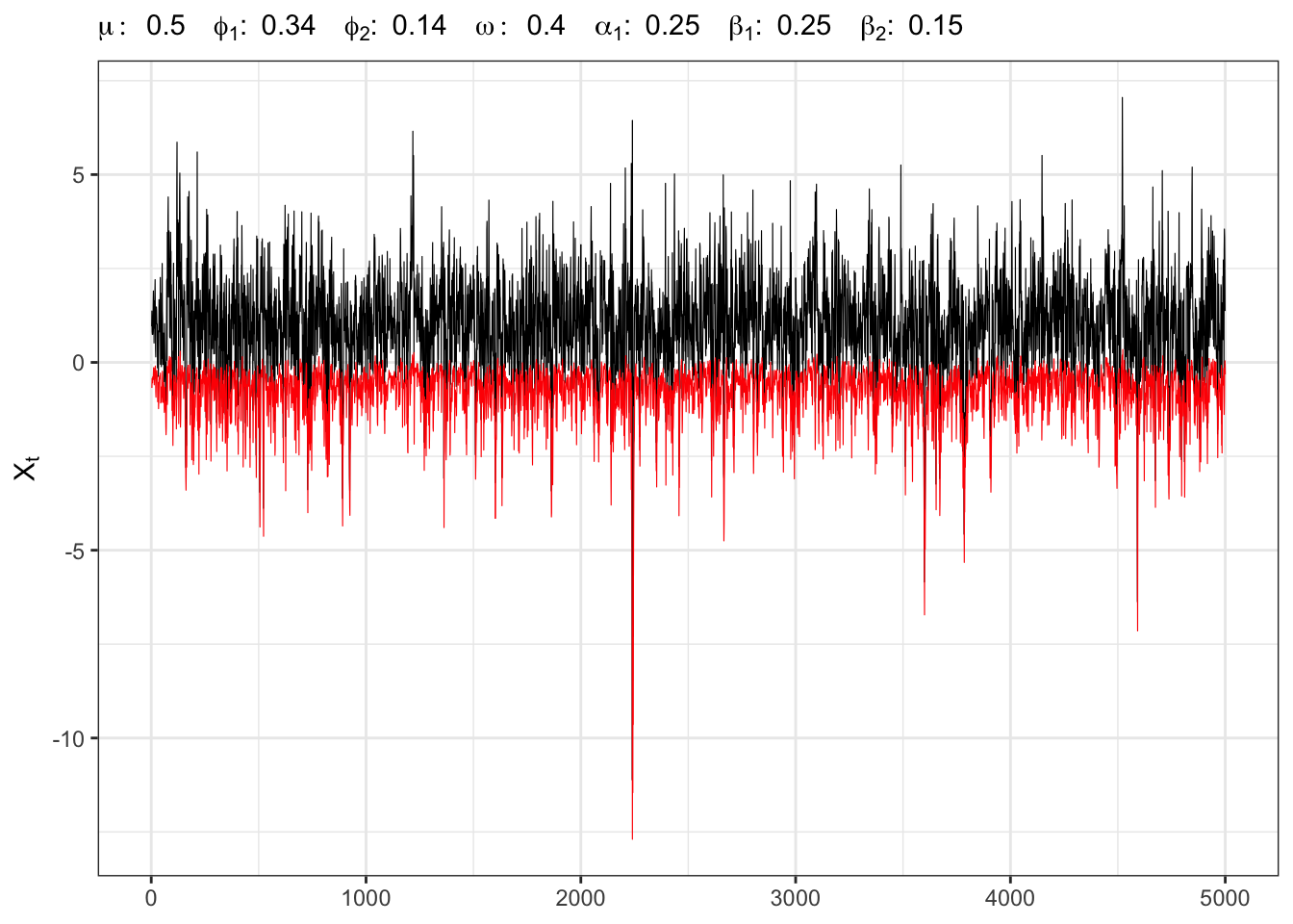
2 Example:
Instead of simulating exactly
AR(2)-GARCH(1,2) simulation and VaR
# ===================== Setups ======================
set.seed(1)   # random seed
ci <- 0.05    # confidence level
t_bar <- 5000 # number of simulations
# parameters
parAR <- c(mu=0.5, phi1 = 0.34, phi1 = 0.14)
parGARCH <- c(omega=0.4, alpha1=0.25,
              beta1=0.25, beta2=0.15)
# long-term std deviation of residuals
sigma_eps <- sqrt(parGARCH[1]/(1-sum(parGARCH[-1])))
# ================== Simulation =====================
# Initial points
Xt <- rep(parAR[1]/(1-sum(parAR[-1])), 3)
sigma <- rep(sigma_eps, 3)
# Simulated residuals
eps <- rt(t_bar, 25)
eps[1:3] = eps[1:3]*sigma_eps
# Value at Risk
q_alpha = qnorm(ci)
VaR = c(0)
for(t in 3:t_bar){
  # AR component
  Xt[t] <- parAR[1] + parAR[2]*Xt[t-1] + parAR[3]*Xt[t-2]
  # ARCH component
  sigma[t] <- parGARCH[1] + parGARCH[2]*eps[t-1]^2
  # GARCH component
  sigma[t] <- sigma[t] + parGARCH[3]*sigma[t-1]^2 + parGARCH[4]*sigma[t-2]^2
  sigma[t] <- sqrt(sigma[t])
  # Simulated residuals
  eps[t] <- sigma[t]*eps[t]
  # Simulated value at risk
  VaR[t] <- Xt[t] + sigma[t]*q_alpha
  # Simulated time series
  Xt[t] <- Xt[t] + eps[t]
}
# ===================== Plot ======================
# GARCH(1,1) simulation
ggplot()+
  geom_line(aes(1:t_bar, Xt), size = 0.2)+
  geom_line(aes(1:t_bar, VaR), size = 0.2, color = "red")+
  theme_bw()+
  labs(x = NULL, y = TeX("$X_t$"),
       subtitle = TeX(paste0("$\\mu:\\;", parAR[1],
                             "\\;\\; \\phi_{1}:\\;", parAR[2],
                             "\\;\\; \\phi_{2}:\\;", parAR[3],
                             "\\;\\; \\omega:\\;", parGARCH[1],
                             "\\;\\; \\alpha_{1}:\\;", parGARCH[2],
                             "\\;\\; \\beta_{1}:\\;", parGARCH[3],
                             "\\;\\; \\beta_{2}:\\;", parGARCH[4],
                             "$")))
NV test Student-
# ======================================
# Violation of the VaR
vt <- ifelse(Xt < VaR, 1, 0)
vt[1:3] <- 0
# Theoric variance
v_theoric <- ci*(1-ci)
# Empiric variance
v_empiric <- (sum(vt)/t_bar)*(1 - sum(vt)/t_bar)
# Standardized number of violations
Nt <- sum((vt - ci)/sqrt(v_theoric))
# Statistic test (NV_1)
NV1 <- (1/sqrt(t_bar))*Nt
# Statistic test (NV_2)
NV2 <- (sqrt(v_theoric)/sqrt(v_empiric))*NV1
# Rejection level
t_alpha <- qnorm(ci/2)
# =============== Kable ===============
kab <- dplyr::tibble(
  n = t_bar,
  alpha = paste0(format(ci*100, digits = 3), "%"),
  alpha_hat = paste0(format(sum(vt)/t_bar*100, digits = 3), "%"),
  t_alpha_dw = t_alpha,
  NV1 = NV1,
  NV2 = NV2,
  t_alpha_up = -t_alpha,
  H01 = ifelse(NV1 > t_alpha_up | NV1 < t_alpha_dw, "Rejected", "Non-Rejected"),
  H02 = ifelse(NV2 > t_alpha_up | NV2 < t_alpha_dw, "Rejected", "Non-Rejected")
)  %>%
  dplyr::mutate_if(is.numeric, format, digits = 4, scientific = FALSE)
colnames(kab) <- c("$$n$$", "$$\\alpha$$", "$$\\frac{N_n}{n}$$", "$$-t_{\\alpha/2}$$",
                   "$$NV_1$$", "$$NV_2$$", "$$t_{\\alpha/2}$$", "$$H_0(NV_1)$$", "$$H_0(NV_2)$$")
knitr::kable(kab, booktabs = TRUE ,escape = FALSE, align = 'c')%>%
kableExtra::row_spec(0, color = "white", background = "green") 3 Example:
Instead of simulating exactly
AR(2)-GARCH(1,2) simulation and VaR
# ==================== Setups =====================
set.seed(1)   # random seed
ci <- 0.05    # confidence level
t_bar <- 1000 # number of simulations
# parameters
parAR <- c(mu=0.5, phi1 = 0.34, phi1 = 0.14)
parGARCH <- c(omega=0.4, alpha1=0.25,
              beta1=0.25, beta2=0.15)
# quasi long-term std deviation of residuals
sigma_eps <- sqrt(parGARCH[1]/(1-sum(parGARCH[-1])))
# ================== Simulation ===================
set.seed(1)
# Initial points
Xt <- rep(parAR[1]/(1-sum(parAR[-1])), 3)
mu <- rep(parAR[1]/(1-sum(parAR[-1])), 3)
sigma <- rep(sigma_eps, 3)
# Simulated residuals
eps <- rt(t_bar, 5)
eps[1:3] <- eps[1:3]*sigma_eps
# Value at Risk
q_alpha = qnorm(ci)
VaR = c(0)
for(t in 3:t_bar){
  # AR component
  mu[t] <- parAR[1] + parAR[2]*Xt[t-1] + parAR[3]*Xt[t-2]
  # ARCH component
  sigma[t] <- parGARCH[1] + parGARCH[2]*eps[t-1]^2
  # GARCH component
  sigma[t] <- sigma[t] + parGARCH[3]*sigma[t-1]^2 + parGARCH[4]*sigma[t-2]^2
  sigma[t] <- sqrt(sigma[t])
  # Simulated residuals
  eps[t] <- sigma[t]*eps[t]
  # Simulated value at risk
  VaR[t] <- mu[t] + sigma[t]*q_alpha
  # Simulated time series
  Xt[t] <- mu[t] + eps[t]
}
# Empirical quantile
q_alpha_emp <- quantile(eps/sigma, probs = ci)
VaR_emp <- mu + sigma*q_alpha_emp

# ===================== Plot ======================
# GARCH(1,1) simulation
ggplot()+
  geom_line(aes(1:t_bar, Xt), size = 0.2)+
  geom_line(aes(1:t_bar, VaR), size = 0.2, color = "red")+
  geom_line(aes(1:t_bar, VaR_emp), size = 0.2, color = "blue")+
  theme_bw()+
  labs(x = NULL, y = TeX("$X_t$"),
       subtitle = TeX(paste0("$\\mu:\\;", parAR[1],
                             "\\;\\; \\phi_{1}:\\;", parAR[2],
                             "\\;\\; \\phi_{2}:\\;", parAR[3],
                             "\\;\\; \\omega:\\;", parGARCH[1],
                             "\\;\\; \\alpha_{1}:\\;", parGARCH[2],
                             "\\;\\; \\beta_{1}:\\;", parGARCH[3],
                             "\\;\\; \\beta_{2}:\\;", parGARCH[4],
                             "$")))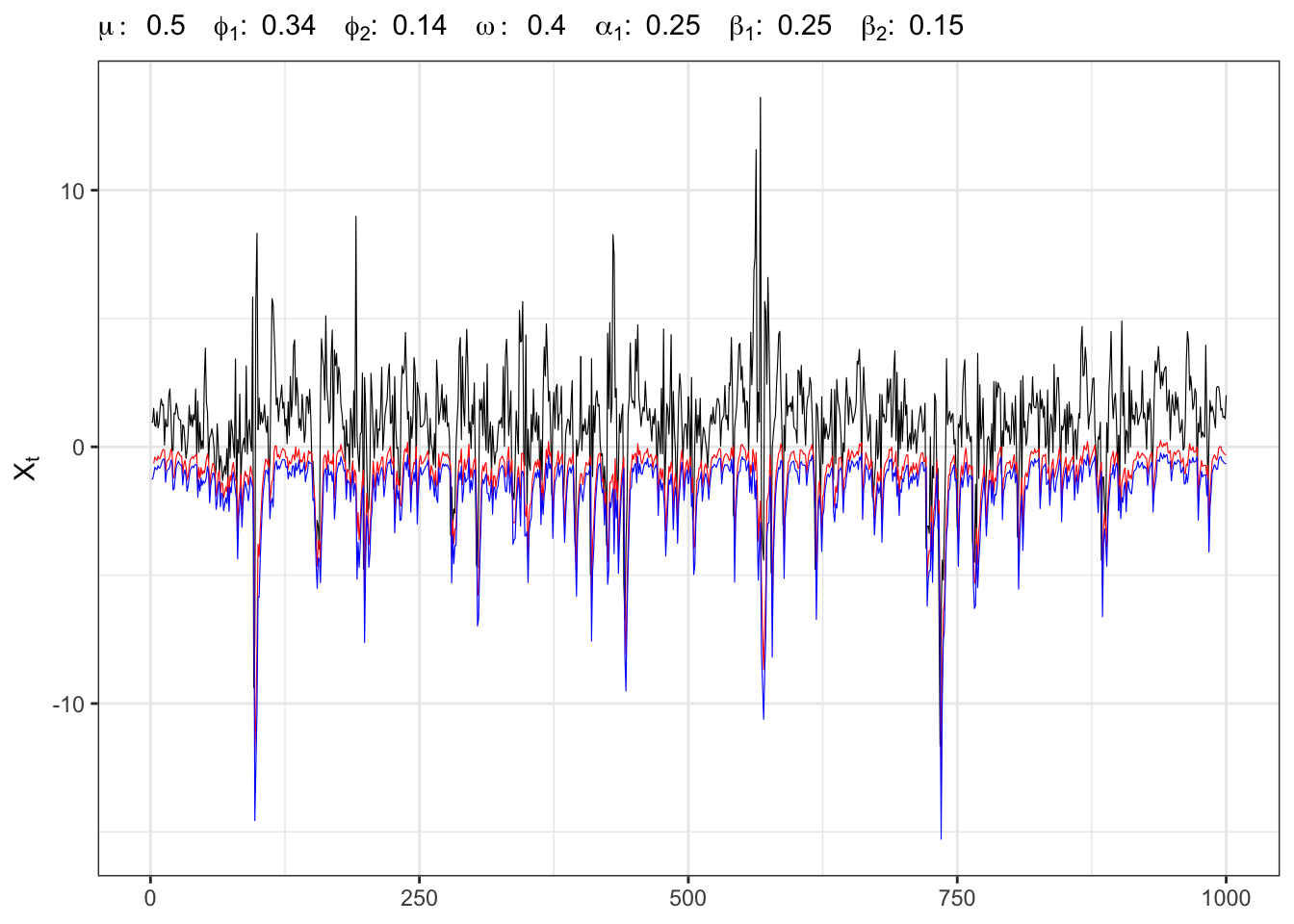
Computing the test on the normal quantile gives a rejection of the null hypothesis
Theoric NV test Student-
# ======================================
# Violation of the VaR
vt <- ifelse(Xt < VaR, 1, 0)
vt[1:3] <- 0
# Theoric variance
v_theoric <- ci*(1-ci)
# Empiric variance
v_empiric <- (sum(vt)/t_bar)*(1 - sum(vt)/t_bar)
# Standardized number of violations
Nt <- sum((vt - ci)/sqrt(v_theoric))
# Statistic test (NV_1)
NV1 <- (1/sqrt(t_bar))*Nt
# Statistic test (NV_2)
NV2 <- (sqrt(v_theoric)/sqrt(v_empiric))*NV1
# Rejection level
t_alpha <- qnorm(ci/2)
# =============== Kable ===============
kab <- dplyr::tibble(
  n = t_bar,
  alpha = paste0(format(ci*100, digits = 3), "%"),
  alpha_hat = paste0(format(sum(vt)/t_bar*100, digits = 3), "%"),
  t_alpha_dw = t_alpha,
  NV1 = NV1,
  NV2 = NV2,
  t_alpha_up = -t_alpha,
  H01 = ifelse(NV1 > t_alpha_up | NV1 < t_alpha_dw, "Rejected", "Non-Rejected"),
  H02 = ifelse(NV2 > t_alpha_up | NV2 < t_alpha_dw, "Rejected", "Non-Rejected")
)  %>%
  dplyr::mutate_if(is.numeric, format, digits = 4, scientific = FALSE)
colnames(kab) <- c("$$n$$", "$$\\alpha$$", "$$\\frac{N_n}{n}$$", "$$-t_{\\alpha/2}$$",
                   "$$NV_1$$", "$$NV_2$$", "$$t_{\\alpha/2}$$", "$$H_0(NV_1)$$", "$$H_0(NV_2)$$")
knitr::kable(kab, booktabs = TRUE ,escape = FALSE, align = 'c')%>%
kableExtra::row_spec(0, color = "white", background = "green") Setting
4 VaR for
From the series of close prices
library(rugarch)
ci <- 0.05    # confidence level
# library(binancer) download prices
load("../../../databases/data/temporary/crypto_prices.RData")
#btcusdt <- binancer::binance_klines("BTCUSDT", api = "spot", interval = "1d",
#                                    from = "2018-01-01", to = Sys.Date())
# log close prices
btcusdt$log_Pt <- log(btcusdt$close)
# log returns
btcusdt$Rt <- c(0, diff(btcusdt$log_Pt))
# In sample estimate
data <- dplyr::filter(btcusdt, date <= as.POSIXct("2024-01-01"))
# Test
data_test <- dplyr::filter(btcusdt, date >= as.POSIXct("2023-12-01"))
fit GARCH(2,3)
# GARCH Model
# Variance specification
GARCH_spec <- rugarch::ugarchspec(
    variance.model = list(model = "sGARCH", garchOrder = c(2,3), external.regressors = NULL),
    mean.model = list(armaOrder = c(0,0), include.mean = FALSE), distribution.model = "norm")
# Fitted model
GARCH_model <- rugarch::ugarchfit(data = data$Rt, spec = GARCH_spec, out.sample = 0)
# Fitted variance
data$sigma2 <- GARCH_model@fit$var
# Fitted standard deviation
data$sigma <- sqrt(data$sigma2)
# Standardized residuals
data$ut <- data$Rt/data$sigma

kab <- as_tibble(t(as_tibble(GARCH_model@fit$coef)))%>%
  dplyr::mutate_if(is.numeric, format, digits = 4, scientific = FALSE)
colnames(kab) <- c("$$\\omega$$", "$$\\alpha_1$$", "$$\\alpha_2$$",
                   "$$\\beta_1$$", "$$\\beta_2$$", "$$\\beta_3$$")
knitr::kable(kab, booktabs = TRUE ,escape = FALSE, align = 'c')%>%
kableExtra::row_spec(0, color = "white", background = "green") 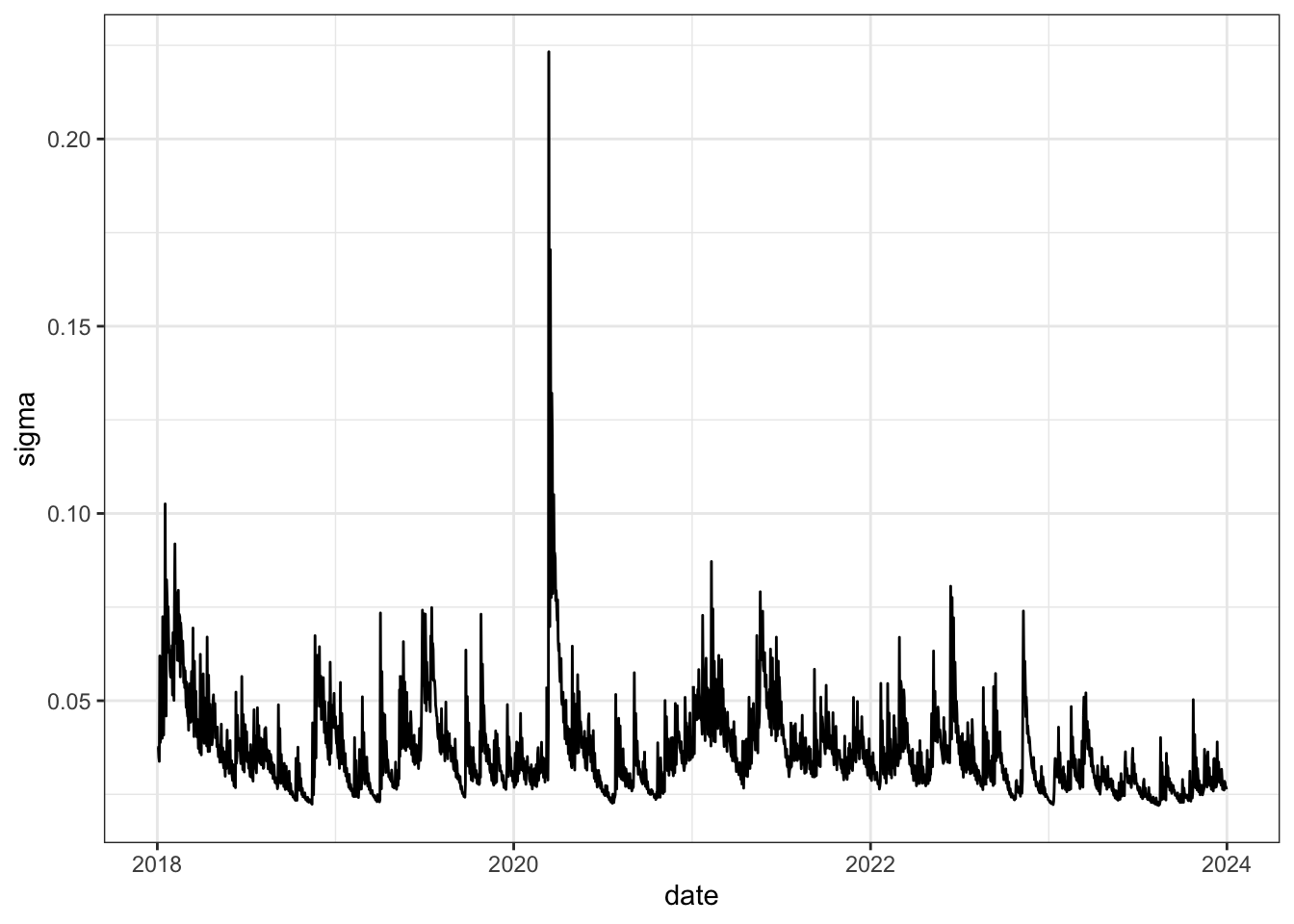
Empiric vs theoric VaR on (
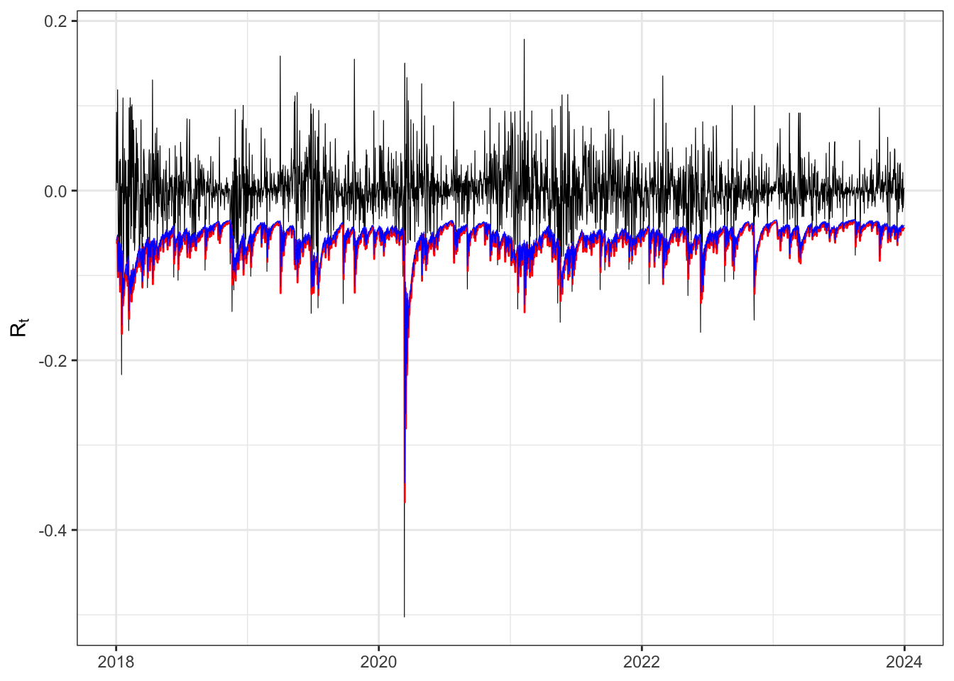
Empiric NV test (
# ======================================
Xt <- data$Rt
t_bar <- nrow(data)
# Violation of the VaR
vt <- ifelse(Xt < VaR, 1, 0)
vt[1:3] <- 0
# Theoric variance
v_theoric <- ci*(1-ci)
# Empiric variance
v_empiric <- (sum(vt)/t_bar)*(1 - sum(vt)/t_bar)
# Standardized number of violations
Nt <- sum((vt - ci)/sqrt(v_theoric))
# Statistic test (NV_1)
NV1 <- (1/sqrt(t_bar))*Nt
# Statistic test (NV_2)
NV2 <- (sqrt(v_theoric)/sqrt(v_empiric))*NV1
# Rejection level
t_alpha <- qnorm(ci/2)
# =============== Kable ===============
kab <- dplyr::tibble(
  n = t_bar,
  alpha_hat = paste0(format(sum(vt)/t_bar*100, digits = 3), "%"),
  t_alpha_dw = t_alpha,
  NV1 = NV1,
  NV2 = NV2,
  t_alpha_up = -t_alpha,
  H01 = ifelse(NV1 > t_alpha_up | NV1 < t_alpha_dw, "Rejected", "Non-Rejected"),
  H02 = ifelse(NV2 > t_alpha_up | NV2 < t_alpha_dw, "Rejected", "Non-Rejected")
)  %>%
  dplyr::mutate_if(is.numeric, round, digits = 4)
colnames(kab) <- c("$$n$$", "$$\\frac{N_n}{n}$$", "$$-t_{\\alpha/2}$$",
                   "$$NV_1$$", "$$NV_2$$", "$$t_{\\alpha/2}$$", "$$H_0(NV_1)$$", "$$H_0(NV_2)$$")
knitr::kable(kab, booktabs = TRUE ,escape = FALSE, align = 'c')%>%
kableExtra::row_spec(0, color = "white", background = "green") GARCH(2,3) simulation (
# ==================== Setups =====================
set.seed(3959) # random seed
parAR <- c(mu=0, phi1=0, phi2=0) # AR parameters
parGARCH <- GARCH_model@fit$coef # GARCH parameters
# long-term std deviation of residuals
sigma_eps <- sqrt(parGARCH[1]/(1-sum(parGARCH[-1])))
# ================== Simulation ===================
# Initial points
Xt <- data_test$Rt
# number of simulations
t_bar <- length(Xt)
mu <- rep(parAR[1]/(1-sum(parAR[-1])), 4)
sigma <- rep(sigma_eps, 4)
# Simulated residuals
eps <- rnorm(t_bar)
eps[1:4] = eps[1:4]*sigma[1]
# Value at Risk
q_alpha = qnorm(ci)
VaR = c(0)
for(t in 4:t_bar){
  # AR component
  mu[t] <- parAR[1] + parAR[2]*Xt[t-1] + parAR[3]*Xt[t-2]
  # ARCH component
  sigma[t] <- parGARCH[1] + parGARCH[2]*eps[t-1]^2 + parGARCH[3]*eps[t-2]^2
  # GARCH component
  sigma[t] <- sigma[t] + parGARCH[4]*sigma[t-1]^2 + parGARCH[5]*sigma[t-2]^2 + parGARCH[6]*sigma[t-3]^2
  sigma[t] <- sqrt(sigma[t])
  # Simulated residuals
  eps[t] <- sigma[t]*eps[t]
  # Simulated value at risk
  VaR[t] <- mu[t] + sigma[t]*q_alpha
  # Simulated time series
  Xt[t] <- mu[t] + eps[t]
}
# Empirical quantile
q_alpha_emp <- quantile(eps/sigma, probs = ci)
VaR_emp <- mu + sigma*q_alpha_emp

# ===================== Plot ======================
# GARCH(2,3) simulation
ggplot()+
  geom_line(aes(data_test$date, data_test$close[4]*cumprod(exp(Xt)), color = "sim"), size = 0.2)+
  geom_line(aes(data_test$date, data_test$close[4]*cumprod(exp(data_test$Rt)), color = "emp"), size = 0.2)+
  scale_color_manual(values = c(sim = "red", emp = "black"),
                     labels = c(sim = "Simulated", emp = "Empiric"))+
  theme_bw()+
  theme(legend.position = "top")+
  labs(x = NULL, y = "BTC-USDT", color = NULL)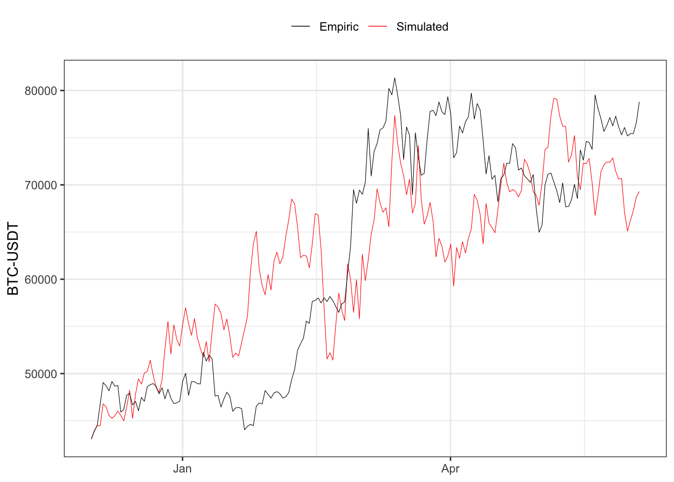
Citation
@online{sartini2024,
  author = {Sartini, Beniamino},
  title = {Tests on the {Value} at {Risk}},
  date = {2024-05-01},
  url = {https://greenfin.it/statistics/tests/var-tests.html},
  langid = {en}
}