Gaussian mixture

Author
Affiliation

Beniamino Sartini

University of Bologna

Published

May 1, 2024

Modified

July 25, 2024

Setup
library(dplyr)
# required for figures  
library(ggplot2)
library(gridExtra)
# required for render latex 
library(backports)
library(latex2exp)
# required for render tables
library(knitr)
library(kableExtra)
# Random seed 
set.seed(1)

Let’s consider a linear combination of a Bernoulli and two normal random variables, all assumed to be independent, i.e. \[ X \sim B \cdot Z_1 + (1-B) \cdot Z_2 \text{,} \tag{1}\] or in compact form \(X \sim GM(\mu_1, \mu_2, \sigma_1^2,\sigma_2^2, p)\). Formally, \(B \sim \text{Ber}(p)\) is a Bernoulli while \(Z_1 = \mathcal{N}(\mu_1, \sigma_1^2)\) and \(Z_2 = \mathcal{N}(\mu_2, \sigma_2^2)\) are two independent Gaussian random variables.

Gaussian mixture simulation
# ================== Setups ==================
t_bar <- 5000 # number of steps ahead  
# parameters
par <- c(mu1=-2,mu2=2,sd1=1,sd2=1,p=0.5) 
# ============================================
# Gaussian mixture simulation 
N_1 <- rnorm(t_bar, mean = par[1], sd = par[3])
N_2 <- rnorm(t_bar, mean = par[2], sd = par[4])
B <- rbinom(t_bar, 1, prob = par[5])
Xt <- B*N_1 + (1 - B)*N_2
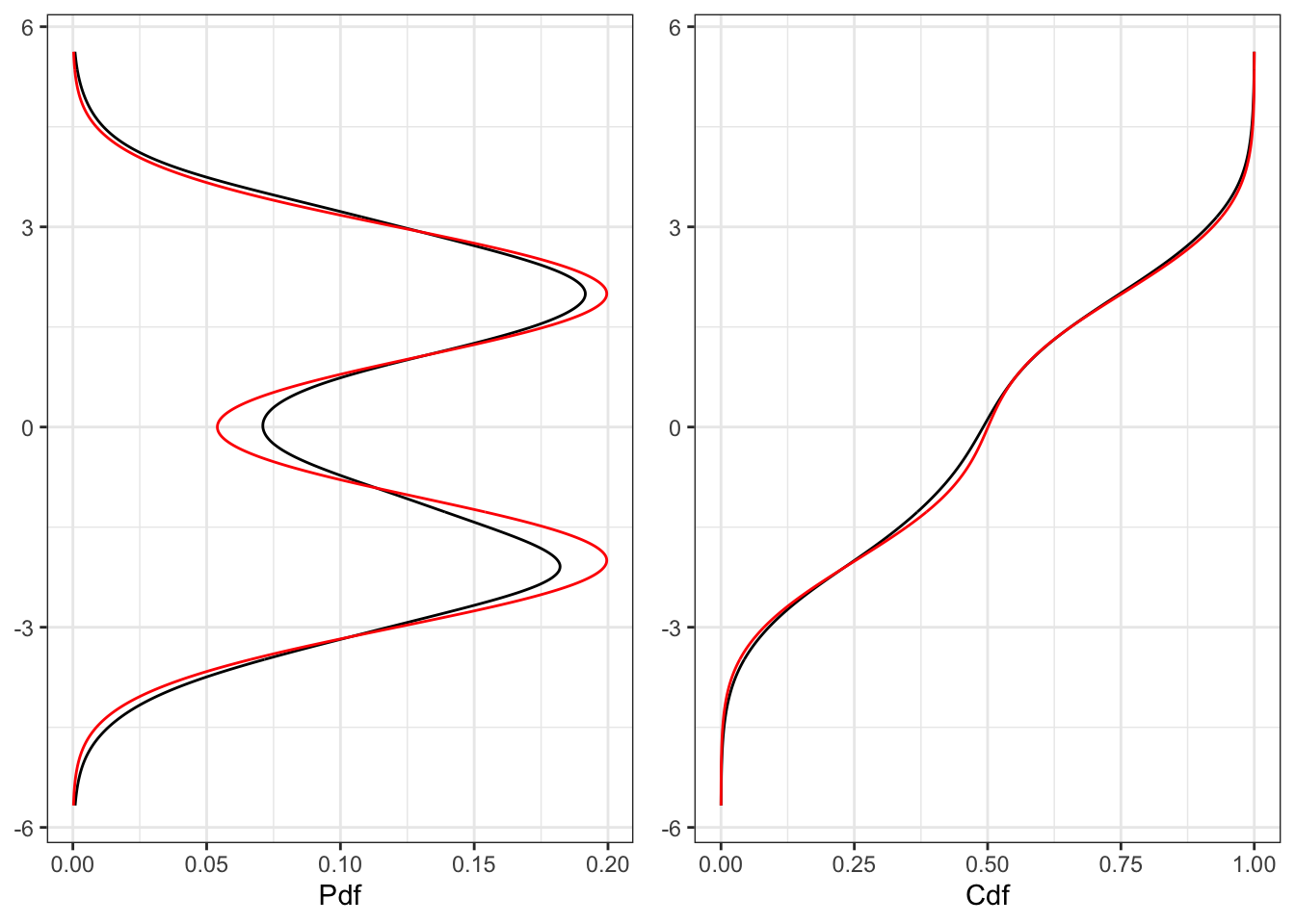
# Empiric pdf and cdf  
ker <- density(Xt, from = min(Xt), to = max(Xt))
ker$cdf_emp <- cumsum(ker$y/sum(ker$y))
# Components normal pdf 
ker$pdf_Z1 <- dnorm(ker$x, mean = par[1], sd = par[3]) 
ker$pdf_Z2 <- dnorm(ker$x, mean = par[2], sd = par[4])
# Mixture pdf and cdf 
ker$pdf <- par[5]*ker$pdf_Z1 + (1-par[5])*ker$pdf_Z2
ker$cdf <- cumsum(ker$pdf/sum(ker$pdf))
# =================== Plot ===================
# Plot trajectory
plot_gm <- ggplot()+
  geom_point(aes(1:t_bar, Xt), alpha = exp(-0.00009*t_bar))+
  labs(x = "t", y = TeX("$X_t$"))+
  theme_bw()
# Plot pdf 
plot_pdf <- ggplot()+
  geom_line(aes(ker$x, ker$y))+
  geom_line(aes(ker$x, ker$pdf), color = "red")+
  labs(x = NULL, y = "Pdf")+
  theme_bw()+
  coord_flip()
# Plot cdf 
plot_cdf <- ggplot()+
  geom_line(aes(ker$x, ker$cdf_emp))+
  geom_line(aes(ker$x, ker$cdf), color = "red")+
  labs(x = NULL, y = "Cdf")+
  theme_bw()+
  coord_flip()
plot_gm
gridExtra::grid.arrange(plot_pdf, plot_cdf, ncol = 2)
(a) Simulation.
(b) Pdf and Cdf.
Figure 1: Gaussian Mixture simulation and density function with parameters \(\mu_1 = -2\), \(\mu_2 = 2\), \(\sigma_1 = 1\), \(\sigma_2 = 1\) and \(p = 0.5\).

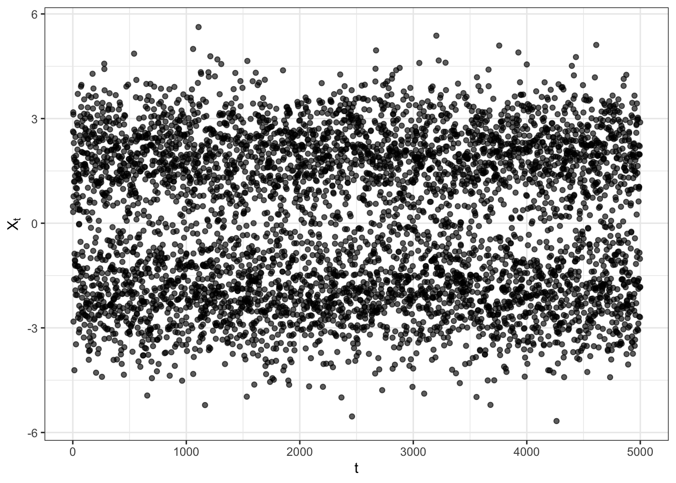
1 Distribution and density

The distribution function of a Gaussian mixture reads explicitely as: \[ F_{X}(x) = p \cdot \Phi\left(\frac{x - \mu_1}{\sigma_1}\right) + (1-p) \cdot \Phi\left(\frac{x - \mu_2}{\sigma_2}\right) \text{,} \tag{2}\] where \(\Phi\) is the cumulative distribution function of a standard normal random variable. Taking the derivative, it can be easily shown that the density function reads: \[ f_{X}(x) = p \cdot \phi\left(\frac{x - \mu_1}{\sigma_1}\right) + (1-p) \cdot \phi\left(\frac{x - \mu_2}{\sigma_2}\right) \text{.} \tag{3}\] where \(\phi\) is the density function of a standard normal random variable.

dnorm_mix <- function(params) {
  # parameters
  mu1 = params[1]
  mu2 = params[2]
  sd1 = params[3]
  sd2 = params[4]
  p = params[5]
  function(x, log = FALSE){
    probs <- p*stats::dnorm(x, mean = mu1, sd = sd1) + (1-p)*stats::dnorm(x, mean = mu2, sd = sd2)
    if (log) {
      probs <- base::log(probs)
    }
    return(probs)
  }
}

Proof. The distribution function of a Gaussian Mixture is defined as: \[ F_{X}(y) = \mathbb{P}(X \le y) = \mathbb{E}\{\mathbb{1}_{X \le x}\} \] Hence, we can rewrite it in terms of conditional expectation with respect to \(B\), i.e.  \[ \begin{aligned} F_{X}(y) & {} = \mathbb{E}\{\mathbb{1}_{X \le x}|B\} = \\ & = \mathbb{E}\{\mathbb{1}_{X \le x}|B = 0\}\mathbb{P}(B = 0) + \mathbb{E}\{\mathbb{1}_{X \le x}|B = 1\}\mathbb{P}(B = 1) = \\ & = p \cdot \mathbb{P}(Z_1 \le x) + (1-p) \cdot \mathbb{P}(Z_2 \le x) \end{aligned} \] Hence, standardizing the normal random variable we obtain, \[ F_{X}(x) = p \cdot \Phi\left(\frac{x - \mu_1}{\sigma_1}\right) + (1-p) \cdot \Phi\left(\frac{x - \mu_2}{\sigma_2}\right) \text{.} \] where \(\Phi\) denotes the distribution function of a standard normal. Knowing that \(f_X(x) = \frac{dF_{X}(x)}{dx}\) and that \(\phi_X(x) = \frac{d\Phi(x)}{dx}\), where \(\phi\) is the density function of a standard normal we obtain the result, i.e. \[ f_{X}(x) = p \cdot \phi\left(\frac{x - \mu_1}{\sigma_1}\right) + (1-p) \cdot \phi\left(\frac{x - \mu_2}{\sigma_2}\right) \text{.} \]

2 Moments

Given that \(Z_1\), \(Z_2\) and \(B\) are independent, the expectation can be computed as: \[ \mathbb{E}\{X\} = p \mu_1 + (1-p) \mu_2 \] The second moment is computed as: \[ \mathbb{E}\{X^2\} = p (\mu_1^2 + \sigma_1^2) + (1-p) (\mu_2^2 + \sigma_2^2) \] Hence, the variance reads: \[ \begin{aligned} \mathbb{V}\{X\} = p(1-p)(\mu_1 - \mu_2)^2 + \sigma_1^2 p + \sigma_2^2 (1-p) \end{aligned} \]

Proof. Given that \(Z_1\), \(Z_2\) and \(B\) are independent, the expectation can be computed as: \[ \begin{aligned} \mathbb{E}\{X\} {} & = \mathbb{E}\{\mathbb{E}\{X|B\}\} = \\ & = \mathbb{E}\{X|B = 1\}\mathbb{P}(B=1) + \mathbb{E}\{X|B = 0\}\mathbb{P}(B=0) = \\ & = p \mathbb{E}\{Z_1\} + (1-p) \mathbb{E}\{Z_2\} = \\ & = p \mu_1 + (1-p) \mu_2 \end{aligned} \] The second moment is computed similarly to the first one, i.e.  \[ \begin{aligned} \mathbb{E}\{X^2\} {} & = \mathbb{E}\{\mathbb{E}\{X^2|B\}\} = \\ & = \mathbb{E}\{X^2|B = 1\}\mathbb{P}(B=1) + \mathbb{E}\{X^2|B = 0\}\mathbb{P}(B=0) = \\ & = \mathbb{E}\{B\} \mathbb{E}\{Z_1^2\} + \mathbb{E}\{1-B\} \mathbb{E}\{Z_2^2\} = \\ & = p \mathbb{E}\{Z_1^2\} + (1-p) \mathbb{E}\{Z_2^2\} = \\ & = p (\mu_1^2 + \sigma_1^2) + (1-p) (\mu_2^2 + \sigma_2^2) \end{aligned} \] The variance, by definition, is given by: \[ \mathbb{V}\{X\} = \mathbb{E}\{X^2\} - \mathbb{E}\{X\}^2 \] where the first moment squared is \[ \begin{aligned} \mathbb{E}\{X\}^2 {} & = \left[p \mu_1 + (1-p) \mu_2\right]^2 = \\ & = p^2 \mu_1^2 + (1-p)^2 \mu_2^2 + 2p(1-p)\mu_1\mu_2 \end{aligned} \] Hence the variance, \[ \begin{aligned} \mathbb{V}\{X\} {} & = p (\mu_1^2 + \sigma_1^2) + (1-p) (\mu_2^2 + \sigma_2^2) - p^2 \mu_1^2 - (1-p)^2 \mu_2^2 - 2p(1-p)\mu_1\mu_2 = \\ & = {\color{red}{p \mu_1^2}} + {\color{orange}{p \sigma_1^2}} + {\color{darkgreen}{\mu_2^2}} + {\color{orange}{\sigma_2^2}} - {\color{darkgreen}{p\mu_2^2}} - {\color{orange}{p\sigma_2^2}} - {\color{red}{p^2 \mu_1^2}} - {\color{darkgreen}{(1-p)^2\mu_2^2}} - 2p(1-p)\mu_1 \mu_2 = \\ & = {\color{red}{\mu_1^2 p (1-p)}} + {\color{orange}{p \sigma_1^2 + (1-p)\sigma_2^2}} + {\color{darkgreen}{p(1-p) \mu_2^2}} - 2p(1-p)\mu_1 \mu_2 = \\ & = p(1-p)(\mu_1^2 - \mu_2^2 - 2\mu_1\mu_2) + p \sigma_1^2 + (1-p) \sigma_2^2 = \\ & = p(1-p)(\mu_1 - \mu_2)^2 + p \sigma_1^2 + (1-p) \sigma_2^2 \end{aligned} \]

3 Maximum likelihood

Minimizing the negative log-likelihood gives an estimate of the parameters, i.e. \[ \underset{\mu_1, \mu_2, \sigma_1, \sigma_2, p}{\text{argmin}} \left\{\sum_{i = 1}^{t} \log (f_{X}(x_i)) \right\} \text{,} \] or equivalently maximizing the negative log-likelihood, i.e.  \[ \underset{\mu_1, \mu_2, \sigma_1, \sigma_2, p}{\text{argmax}} \left\{-\sum_{i = 1}^{t} \log (f_{X}(x_i)) \right\} \text{.} \]

Maximum likelihood for Gaussian mixture
# Initialize parameters 
init_params <- par*runif(5, 0.3, 1.1)
# Log-likelihood function
log_lik <- function(params, x){
  # Parameters
  mu1 = params[1]
  mu2 = params[2]
  sd1 = params[3]
  sd2 = params[4]
  p = params[5]
  # Ensure that probability is in (0,1)
  if(p > 0.99 | p < 0.01 | sd1 < 0 | sd2 < 0){ s
    return(NA_integer_)
  }
  # Mixture density
  pdf_mix <- dnorm_mix(params)
  # Log-likelihood
  loss <- sum(pdf_mix(x, log = TRUE), na.rm = TRUE)
  return(loss)
}
# Optimal parameters
# fnscale = -1 to maximize (or use negative likelihood)
ml_estimate <- optim(par = init_params, log_lik, 
                     x = Xt, control = list(maxit = 500000, fnscale = -1))
Table 1: Maximum likelihood estimates for a Gaussian Mixture.
Parameter True Estimate Log-lik Bias
$$\mu_1$$ -2.0 -1.9905803 -10332.56 0.0094197
$$\mu_2$$ 2.0 2.0006381 -10332.56 0.0006381
$$\sigma_1$$ 1.0 1.0457653 -10332.56 0.0457653
$$\sigma_2$$ 1.0 1.0033373 -10332.56 0.0033373
$$p$$ 0.5 0.4937459 -10332.56 -0.0062541

4 Moments matching

Let’s fix the parameter of the first component, namely \(\mu_1\) and \(\sigma_1^2\) and a certain probability \(p\). Then let’s compute the sample estimate of the expectation of \(X_t\), i.e. \[ \mathbb{E}\{X\} = \frac{1}{t}\sum_{i = 1}^{t} x_i = \hat{\mu} \] and the sample variance: \[ \mathbb{V}\{X\} = \frac{1}{t}\sum_{i = 1}^{t} (x_i - \hat{\mu})^2 = \hat{\sigma}^2 \] In order to obtain an estimate of the second distribution such that the Gaussian Mixture moments match exactly the sample estimates we solve the system for \(\mu_2\) and \(\sigma_2^2\): \[ \begin{cases} \hat{\mu} = p \mu_1 + (1-p) \mu_2 \\ \hat{\sigma}^2 = p(1-p)(\mu_1 - \mu_2)^2 + \sigma_1^2 p + \sigma_2^2 (1-p) \end{cases} \] which lead to a unique solution, i.e. \[ \begin{aligned} {} & \mu_2 = \frac{\hat{\mu} - p \mu_1}{1-p} \\ & \sigma_2^2 = \frac{\hat{\sigma}^2 - p\sigma_1^2 }{1-p} - p (\mu_1 - \mu_2)^2 \end{aligned} \]

5 Moment generating function

The moment generating function of a Gaussian mixture random variable (Equation 1) reads: \[ M_X(t) = p \cdot \exp\left\{\mu_1 t + \frac{t^2 \sigma_1^2}{2}\right\} + (1-p) \cdot \exp\left\{\mu_2 t + \frac{t^2 \sigma_2^2}{2}\right\} \]

Proof. Applying the definition of moment generating function on a gaussian mixture we obtain: \[ \begin{aligned} M_X(t) & {} = \mathbb{E}\{e^{tX}\} = \\ & = p \cdot \mathbb{E}\{e^{t Z_1}\} + (1-p) \cdot \mathbb{E}\{e^{t Z_2}\} = \\ & = p \cdot M_{Z_1}(t) + (1-p) \cdot M_{Z_1}(t) = \\ & = p \cdot \exp\left\{\mu_1 t + \frac{t^2 \sigma_1^2}{2}\right\} + (1-p) \cdot \exp\left\{\mu_2 t + \frac{t^2 \sigma_2^2}{2}\right\} \end{aligned} \] where \(M_{Z_1}(t)\) and \(M_{Z_2}(t)\) are the moment generating functions of a Gaussian random variable.

6 Esscher transform

The Esscher transform of a Gaussian mixture random variable reads: \[ E_{\theta}\{f_X(x)\} = \tilde{p} \cdot \mathcal{N}(\mu_1 + \theta \sigma_1^2, \sigma_1^2) + (1-\tilde{p}) \cdot \mathcal{N}(\mu_2 + \theta \sigma_2^2, \sigma_2^2) \] where \(\tilde{p}\) are defined as: \[ \tilde{p} = \frac{p M_{Z_1}(\theta)}{p M_{Z_1}(\theta) + (1-p) M_{Z_2}(\theta)} \]

Proof. In general, the Esscher transform of a density function is computed as:
\[ E_{\theta}\{f_X(x)\} = \frac{e^{\theta X} f_X(x)}{M_X(\theta)} = \frac{e^{\theta X} f_X(x)}{\int_{-\infty}^{\infty} e^{\theta X} f_X(x) dx} \] Substituing the density function of a Gaussian mixture we obtain: \[ E_{\theta}\{f_X(x)\} = \frac{e^{\theta X} (p f_{Z_1}(x) + (1-p) f_{Z_2}(x))}{\int_{-\infty}^{\infty} e^{\theta X} (p f_{Z_1}(x) + (1-p) f_{Z_2}(x)) dx} \] Let’s examine the product of the first component: \[ p e^{\theta X} f_{Z_1}(x) = \frac{p e^{\theta x}}{\sqrt{2\pi} \sigma_1} \exp\left\{-\frac{(x-\mu_1)^2}{2\sigma_1^2}\right\} = \frac{1}{\sqrt{2\pi} \sigma_1^2} \exp\left\{-\frac{(x-\mu_1)^2}{2\sigma_1^2} + \theta x \right\} \] In order to rewrite it as the pdf of a normal with mean \((\mu_1 + \theta \sigma_1^2)\), we note that the expansion of such product reads: \[ (x - \mu_1 - \theta \sigma_1^2)^2 = x^2 - 2 x\mu_1 - 2 \theta x \sigma_1^2 + \mu^2 + 2 \mu \theta \sigma_1^2 + \theta^2 \sigma_1^2 \] Hence, let’s add and subtract inside the exponential \(\pm \mu_1 \theta \pm \frac{\theta^2 \sigma_1^2}{2}\), i.e. \[ \begin{aligned} p e^{\theta X} f_{Z_1}(x) & {} = \frac{p}{\sqrt{2\pi} \sigma_1} \exp\left\{-\frac{(x-\mu_1)^2}{2\sigma_1^2} + \theta x - \mu_1 \theta - \frac{\theta^2 \sigma_1^2}{2} \right\} \exp\left\{\mu_1 \theta + \frac{\theta^2 \sigma_1^2}{2}\right\} = \\ & = \frac{p}{\sqrt{2\pi} \sigma_1} \exp\left\{\mu_1 \theta + \frac{\theta \sigma_1^2}{2}\right\} \exp\left\{-\frac{(x-\mu_1 - \theta^2 \sigma_1^2 )^2}{2\sigma_1^2} \right\} \end{aligned} \] Hence let’s collect the first part and the denominator (mgf of the Gaussian mixture in \(\theta\)) and define the new probability: \[ \tilde{p} = \frac{p \exp\left\{\mu_1 \theta + \frac{\theta^2 \sigma_1^2}{2}\right\}}{p \exp\left\{\mu_1 \theta + \frac{\theta^2 \sigma_1^2}{2}\right\} + (1-p) \exp\left\{\mu_2 \theta + \frac{\theta^2 \sigma_2^2}{2}\right\}} \] That can be equivalently written in terms of the moment generating functions, i.e.  \[ \tilde{p}= \frac{p M_{Z_1}(\theta)}{p M_{Z_1}(\theta) + (1-p) M_{Z_2}(\theta)} \] Hence, repeating the same for the second component we obtain that the Esscher transform of a Gaussian mixture is defined as: \[ E_{\theta}\{f_X(x)\} = \tilde{p} \cdot \mathcal{N}(\mu_1 + \theta \sigma_1^2, \sigma_1^2) + (1-\tilde{p}) \cdot \mathcal{N}(\mu_2 + \theta \sigma_2^2, \sigma_2^2) \]

Back to top

Citation

BibTeX citation:
@online{sartini2024,
  author = {Sartini, Beniamino},
  title = {Gaussian Mixture},
  date = {2024-05-01},
  url = {https://greenfin.it/statistics/distributions/gaussian-mixture.html},
  langid = {en}
}
For attribution, please cite this work as:
Sartini, Beniamino. 2024. “Gaussian Mixture.” May 1, 2024. https://greenfin.it/statistics/distributions/gaussian-mixture.html.