Stationarity tests

Author

Affiliation

Beniamino Sartini

University of Bologna

library(dplyr)
library(knitr)
library(kableExtra)
library(ggplot2)

1 Dickey–Fuller test

The Dickey–Fuller test tests the null hypothesis that a unit root is present in an autoregressive (AR) model. The alternative hypothesis is different depending on which version of the test is used, but is usually stationarity or trend-stationarity. Let’s consider an AR(1) model, i.e. \[ x_t = \mu + \delta t + \phi_1 x_{t-1} + u_t \text{,} \tag{1}\] or equivalently \[ \Delta x_t = \mu + \delta t + (1-\phi_1) x_{t-1} + u_t \text{.} \tag{2}\]

The, the Dickey–Fuller hypothesis are: \[ \begin{aligned} {} & H_0: \phi_1 = 1 \;\; (\text{non stationarity}) \\ & H_1: \phi_1 < 1 \;\; (\text{stationarity}) \end{aligned} \] The statistic test is obtained as: \[ DF = \frac{1-\phi_1}{\mathbb{S}d\{1-\phi_1\}} \] However, since the test is done over the residual term rather than raw data, it is not possible to use standard t-distribution to provide critical values. Therefore, the statistic \(DF\) has a specific distribution. In common implementation there are three versions of the test, i.e. standard (\(\psi = 0, \mu = 0\)), drift (\(\mu = 0\)), trend in Equation 1.

2 Augmented Dickey–Fuller test

The augmented Dickey–Fuller is a more general version of the Dickey–Fuller test for a general AR(p) model, i.e.  \[ \Delta x_t = \mu + \delta t + \gamma x_{t-1} + \sum_{i = 1}^{p} \phi_i \Delta x_{t-i} \]

Then, the augmented Dickey–Fuller hypothesis are: \[ \begin{aligned} {} & H_0: \gamma = 0 \;\; (\text{non stationarity}) \\ & H_1: \gamma < 0 \;\; (\text{stationarity}) \end{aligned} \] The statistic test is obtained as: \[ ADF = \frac{\gamma}{\mathbb{S}d\{\gamma\}} \] As in the simpler case, the critical values are computed using a specific table for the Dickey–Fuller test.

3 Kolmogorov-Smirnov test

The Kolmogorov–Smirnov two-sample test (KS test) can be used to test whether two samples came from the same distribution. Let’s define the empirical distribution function \(F_{n}\) of \(n\)-independent and identically distributed ordered observations \(X_{(i)}\) as \[ F_{n}(x) = \frac{1}{n}\sum_{i = 1}^{n} \mathbb{1}_{(-\infty, x]}(X_{(i)}) \text{.} \] The KS statistic quantifies a distance between the empirical distribution function of the sample and the cumulative distribution functions of two samples. The null distribution of this statistic is calculated under the null hypothesis that the samples are drawn from the same distribution, i.e.  \[ \begin{aligned} {} & H_0: X \; \text{stationary} \\ & H_1: X \; \text{non stationary} \end{aligned} \] The statistic test for two samples with dimension \(n_1\) and \(n_2\) is defined as: \[ KS_{n_1, n_2} = \underset{\forall x}{\sup}|F_{n_1}(x) - F_{n_2}(x)| \text{,} \] and for large samples, the null hypothesis is rejected at level \(\alpha\) if: \[ KS_{n_1, n_2} > \sqrt{-\frac{1}{2n_2} \ln\left(\frac{\alpha}{2}\right) \left(1 + \frac{n_2}{n_1}\right)} \text{.} \]

To apply the test in a time series settings, it is possible to random split the original series in two sub samples and apply the test above.

3.1 Example: check stationary

Let’s simulate 500 observations of \(X \sim N(0.4, 1)\), then split the series in a random point and compute the Kolmogorov-Smirnov statistic.

# ============== Setups ==============
set.seed(5) # random seed
ci <- 0.05  # confidence level (alpha)
n <- 500    # number of simulations
# ====================================
# Simulated stationary sample 
x <- rnorm(n, 0.4, 1)
# Random split of the time series
idx_split <- sample(n, 1)
x1 <- x[1:idx_split]
x2 <- x[(idx_split+1):n]
# Number of elements for each sub sample 
n1 <- length(x1)
n2 <- length(x2)
# Grid of values for KS-statistic
grid <- seq(quantile(x, 0.015), quantile(x, 0.985), 0.01)
# Empiric cdfs 
cdf_1 <- ecdf(x1)
cdf_2 <- ecdf(x2)
# KS-statistic 
ks_stat <- max(abs(cdf_1(grid) - cdf_2(grid)))
# Rejection level with probability alpha 
rejection_lev <- sqrt(-0.5*log(ci/2))*sqrt((n1+n2)/(n1*n2))
# ========================== Plot ==========================
y_breaks <- seq(0, 1, 0.2)
y_labels <- paste0(format(y_breaks*100, digits = 2), "%")
grid_max <- grid[which.max(abs(cdf_1(grid) - cdf_2(grid)))]
ggplot()+
  geom_ribbon(aes(grid, ymax = cdf_1(grid), ymin = cdf_2(grid)), 
              alpha = 0.5, fill = "green") +
  geom_line(aes(grid, cdf_1(grid)))+
  geom_line(aes(grid, cdf_2(grid)), color = "red")+
  geom_segment(aes(x = grid_max, xend = grid_max, 
                   y = cdf_1(grid_max), yend = cdf_2(grid_max)), 
               linetype = "solid", color = "magenta")+
  geom_point(aes(grid_max, cdf_1(grid_max)), color = "magenta")+
  geom_point(aes(grid_max, cdf_2(grid_max)), color = "magenta")+
  scale_y_continuous(breaks = y_breaks, labels = y_labels)+
  labs(x = "x", y = "cdf")+
  theme_bw()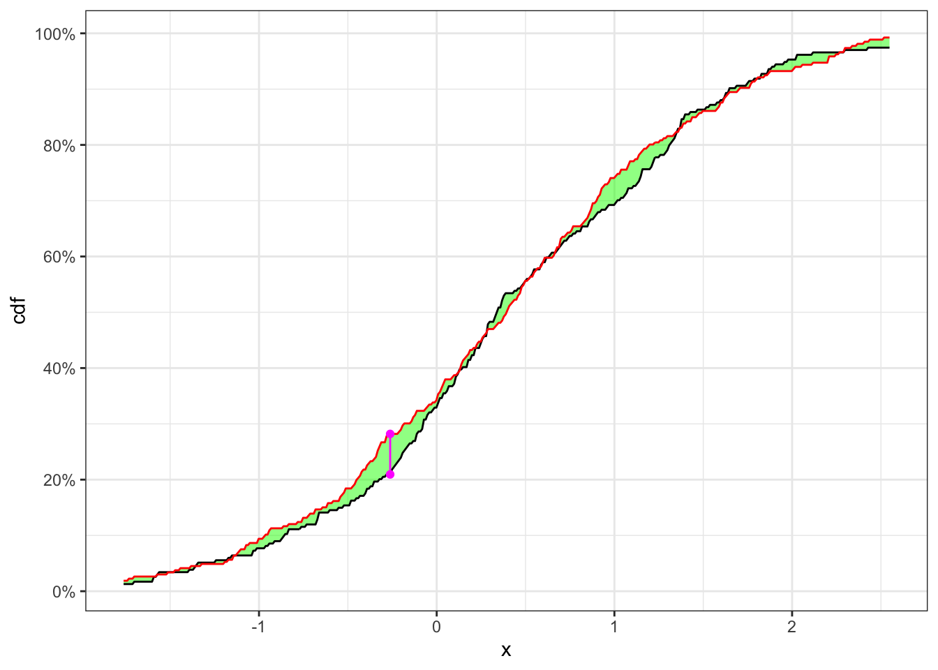

Figure 1: Two samples cdfs and KS-statistic (magenta) for a stationary time series.

Table 1: KS test for a stationary time series.

$$\textbf{Index split}$$	$$\alpha$$	$$n_1$$	$$n_2$$	$$KS_{n_1, n_2}$$	$$\textbf{Critical Level}$$	$$H_0$$
234	5%	234	266	0.07255	0.1217	Non-Rejected

In Table 1 the null hypothesis, i.e. the two samples come from the same distribution, is not reject with the confidence level \(\alpha = 5\%\).

3.2 Example: check non-stationary

Let’s now simulate 250 observations as \(X_1 \sim N(0, 1)\) and the following 250 as \(X_2 \sim N(0.3, 1)\). Then the non-stationary series with a structural break is given by \(X = (X_1, X_2)\). As before, we random split the series and apply the Kolmogorov-Smirnov test.

# ============== Setups ==============
set.seed(2) # random seed
ci <- 0.05  # confidence level (alpha)
n <- 500    # number of simulations
# ====================================
# Simulated non-stationary sample 
x1 <- rnorm(n/2, 0, 1)
x2 <- rnorm(n/2, 0.3, 1)
x <- c(x1, x2)
# Random split of the time series
idx_split <- sample(n, 1)
x1 <- x[1:idx_split]
x2 <- x[(idx_split+1):n]
# Number of elements for each sub sample 
n1 <- length(x1)
n2 <- length(x2)
# Grid of values for KS-statistic
grid <- seq(quantile(x, 0.015), quantile(x, 0.985), 0.01)
# Empiric cdfs 
cdf_1 <- ecdf(x1)
cdf_2 <- ecdf(x2)
# KS-statistic 
ks_stat <- max(abs(cdf_1(grid) - cdf_2(grid)))
# Rejection level  
rejection_lev <- sqrt(-0.5*log(ci/2))*sqrt((n1+n2)/(n1*n2))
# ========================== Plot ==========================
y_breaks <- seq(0, 1, 0.2)
y_labels <- paste0(format(y_breaks*100, digits = 2), "%")
grid_max <- grid[which.max(abs(cdf_1(grid) - cdf_2(grid)))]
ggplot()+
  geom_ribbon(aes(grid, ymax = cdf_1(grid), ymin = cdf_2(grid)), 
              alpha = 0.5, fill = "green") +
  geom_line(aes(grid, cdf_1(grid)))+
  geom_line(aes(grid, cdf_2(grid)), color = "red")+
  geom_segment(aes(x = grid_max, xend = grid_max, 
                   y = cdf_1(grid_max), yend = cdf_2(grid_max)), 
               linetype = "solid", color = "magenta")+
  geom_point(aes(grid_max, cdf_1(grid_max)), color = "magenta")+
  geom_point(aes(grid_max, cdf_2(grid_max)), color = "magenta")+
  scale_y_continuous(breaks = y_breaks, labels = y_labels)+
  labs(x = "x", y = "cdf")+
  theme_bw()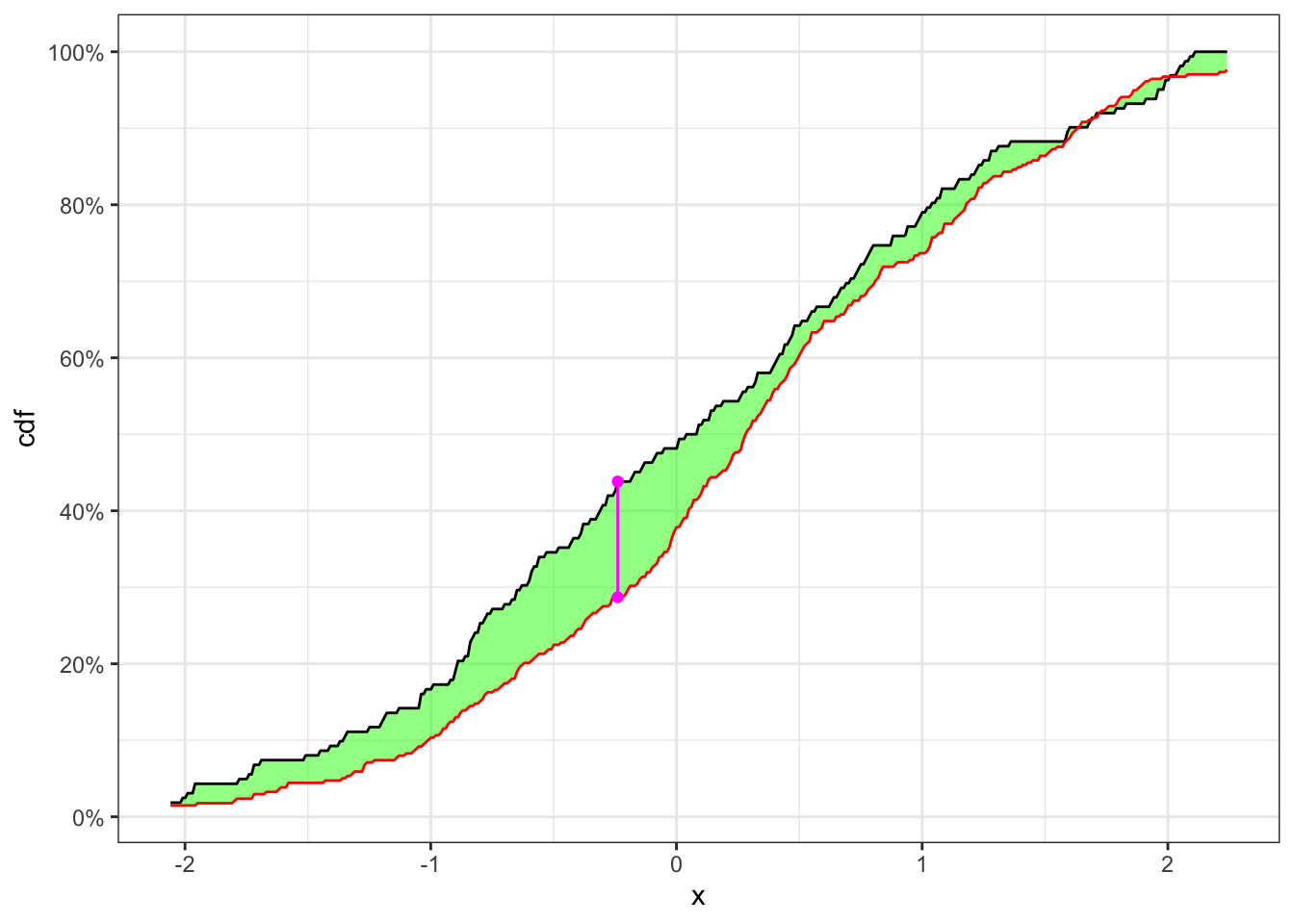

Figure 2: Two samples cdfs and KS-statistic (magenta) for a non-stationary time series.

In Table 2 the null hypothesis, i.e. the two samples come from the same distribution, is reject with a confidence level \(\alpha = 5\%\), hence the two samples come from different distributions.

Table 2: KS test for a non-stationary time series.

$$\textbf{Index split}$$	$$\alpha$$	$$n_1$$	$$n_2$$	$$KS_{n_1, n_2}$$	$$\textbf{Critical Level}$$	$$H_0$$
162	5%	162	338	0.1513	0.1298	Rejected