Tukey functions

1 Tukey’s Bisquare
Plot code
ggplot()+
  geom_line(aes(grid, tukey_bisquare(d[1])(grid), color = "p1"))+
  geom_line(aes(grid, tukey_bisquare(d[2])(grid), color = "p2"))+
  geom_line(aes(grid, tukey_bisquare(d[3])(grid), color = "p3"))+
  geom_line(aes(grid, tukey_bisquare(d[4])(grid), color = "p4"))+
  scale_color_manual(values = c(p1 = "red", p2 = "black", p3 = "green", p4 = "purple"),
                     labels = c(p1 = paste0("d = ", d[1]),
                                p2 = paste0("d = ", d[2]),
                                p3 = paste0("d = ", d[3]),
                                p4 = paste0("d = ", d[4])))+
  theme_bw()+
  scale_x_continuous(breaks = c(min(grid),-d, 0, d, max(grid)))+
  theme(legend.position = "top")+
  labs(x = "x", y = TeX("$\\rho(x; d)$"), color = NULL)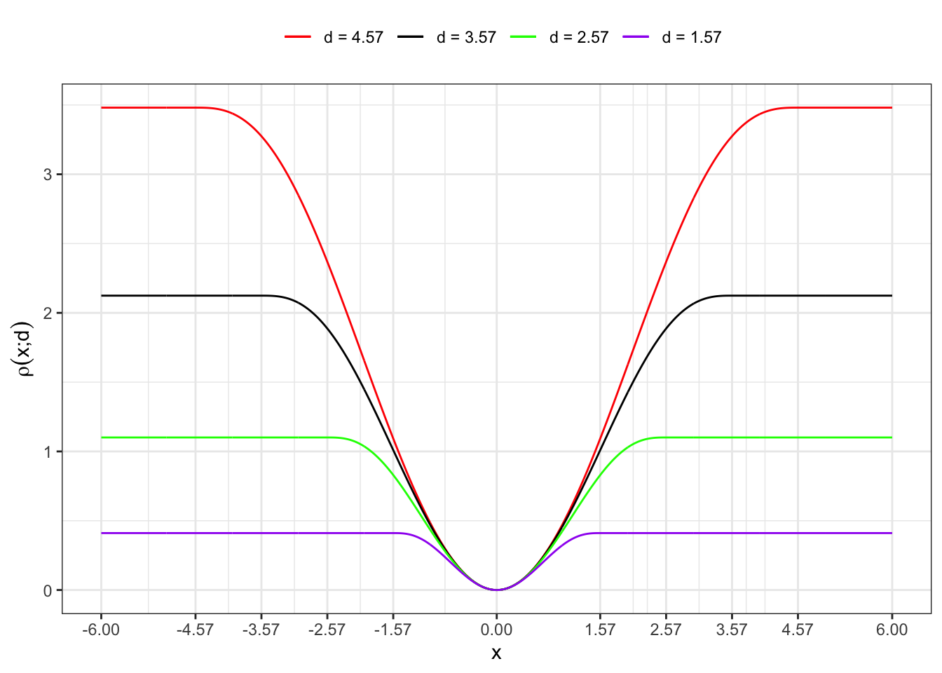
1.1 First derivative
Plot code
ggplot()+
  geom_line(aes(grid, tukey_bisquare_prime(d[1])(grid), color = "p1"))+
  geom_line(aes(grid, tukey_bisquare_prime(d[2])(grid), color = "p2"))+
  geom_line(aes(grid, tukey_bisquare_prime(d[3])(grid), color = "p3"))+
  geom_line(aes(grid, tukey_bisquare_prime(d[4])(grid), color = "p4"))+
  scale_color_manual(values = c(p1 = "red", p2 = "black", p3 = "green", p4 = "purple"),
                     labels = c(p1 = paste0("d = ", d[1]),
                                p2 = paste0("d = ", d[2]),
                                p3 = paste0("d = ", d[3]),
                                p4 = paste0("d = ", d[4])))+
  theme_bw()+
  scale_x_continuous(breaks = c(min(grid),-d, 0, d, max(grid)))+
  theme(legend.position = "top")+
  labs(x = "x", y = TeX("$\\rho^{\\prime}(x; d)$"), color = NULL)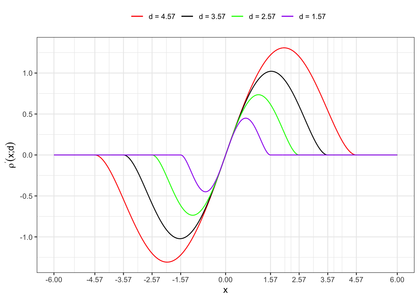
1.2 Second derivative
Plot code
ggplot()+
  geom_line(aes(grid, tukey_bisquare_second(d[1])(grid), color = "p1"))+
  geom_line(aes(grid, tukey_bisquare_second(d[2])(grid), color = "p2"))+
  geom_line(aes(grid, tukey_bisquare_second(d[3])(grid), color = "p3"))+
  geom_line(aes(grid, tukey_bisquare_second(d[4])(grid), color = "p4"))+
  scale_color_manual(values = c(p1 = "red", p2 = "black", p3 = "green", p4 = "purple"),
                     labels = c(p1 = paste0("d = ", d[1]),
                                p2 = paste0("d = ", d[2]),
                                p3 = paste0("d = ", d[3]),
                                p4 = paste0("d = ", d[4])))+
  theme_bw()+
  scale_x_continuous(breaks = c(min(grid),-d, 0, d, max(grid)))+
  theme(legend.position = "top")+
  labs(x = "x", y = TeX("$\\rho^{\\prime\\prime}(x; d)$"), color = NULL)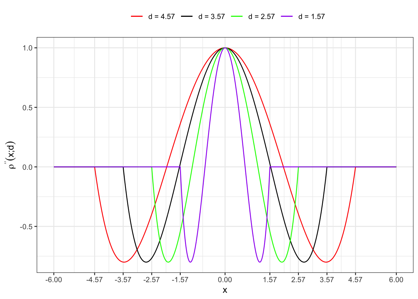
2 Tukey Biweight
Plot code
ggplot()+
  geom_line(aes(grid, tukey_biweight(d[1])(grid), color = "p1"))+
  geom_line(aes(grid, tukey_biweight(d[2])(grid), color = "p2"))+
  geom_line(aes(grid, tukey_biweight(d[3])(grid), color = "p3"))+
  geom_line(aes(grid, tukey_biweight(d[4])(grid), color = "p4"))+
  scale_color_manual(values = c(p1 = "red", p2 = "black", p3 = "green", p4 = "purple"),
                     labels = c(p1 = paste0("d = ", d[1]),
                                p2 = paste0("d = ", d[2]),
                                p3 = paste0("d = ", d[3]),
                                p4 = paste0("d = ", d[4])))+
  theme_bw()+
  scale_x_continuous(breaks = c(min(grid),-d, 0, d, max(grid)))+
  theme(legend.position = "top")+
  labs(x = "x", y = TeX("$\\rho(x; d)$"), color = NULL)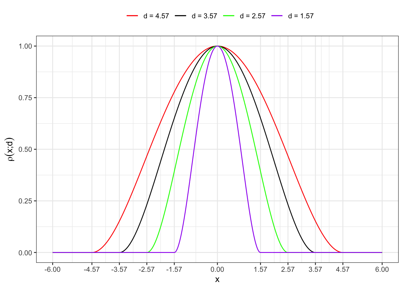
3 Tukey-Beaton Bisquare
Plot code
ggplot()+
  geom_line(aes(grid, tukey_beaton_bisquare(d[1])(grid), color = "p1"))+
  geom_line(aes(grid, tukey_beaton_bisquare(d[2])(grid), color = "p2"))+
  geom_line(aes(grid, tukey_beaton_bisquare(d[3])(grid), color = "p3"))+
  geom_line(aes(grid, tukey_beaton_bisquare(d[4])(grid), color = "p4"))+
  scale_color_manual(values = c(p1 = "red", p2 = "black", p3 = "green", p4 = "purple"),
                     labels = c(p1 = paste0("d = ", d[1]),
                                p2 = paste0("d = ", d[2]),
                                p3 = paste0("d = ", d[3]),
                                p4 = paste0("d = ", d[4])))+
  theme_bw()+
  scale_x_continuous(breaks = c(min(grid),-d, 0, d, max(grid)))+
  theme(legend.position = "top")+
  labs(x = "x", y = TeX("$\\rho(x; d)$"), color = NULL)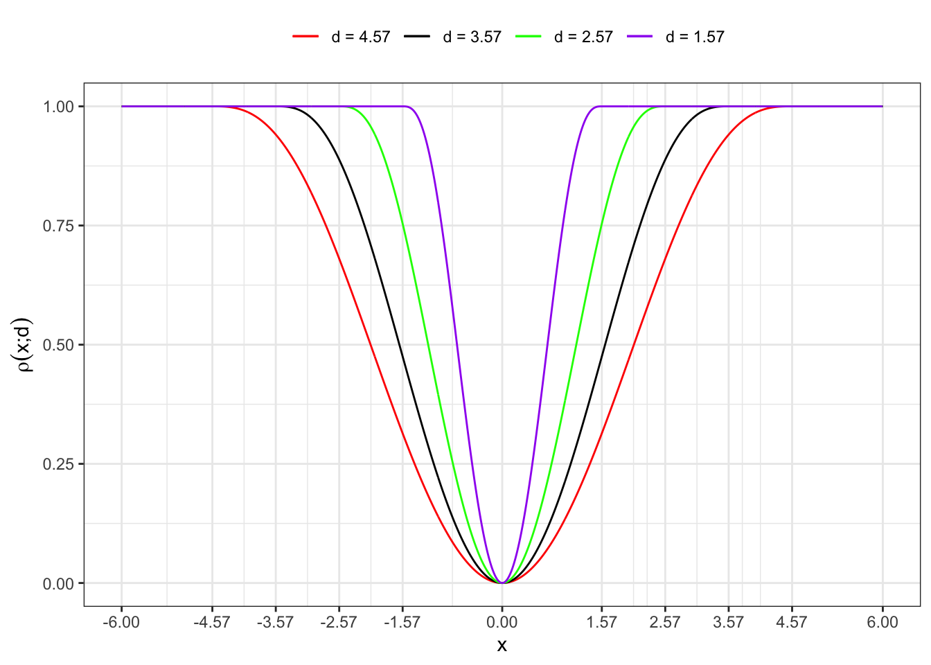
3.1 First derivative
Plot code
ggplot()+
  geom_line(aes(grid, tukey_beaton_prime(d[1])(grid), color = "p1"))+
  geom_line(aes(grid, tukey_beaton_prime(d[2])(grid), color = "p2"))+
  geom_line(aes(grid, tukey_beaton_prime(d[3])(grid), color = "p3"))+
  geom_line(aes(grid, tukey_beaton_prime(d[4])(grid), color = "p4"))+
  scale_color_manual(values = c(p1 = "red", p2 = "black", p3 = "green", p4 = "purple"),
                     labels = c(p1 = paste0("d = ", d[1]),
                                p2 = paste0("d = ", d[2]),
                                p3 = paste0("d = ", d[3]),
                                p4 = paste0("d = ", d[4])))+
  theme_bw()+
  scale_x_continuous(breaks = c(min(grid),-d, 0, d, max(grid)))+
  theme(legend.position = "top")+
  labs(x = "x", y = TeX("$\\rho^{\\prime}(x; d)$"), color = NULL)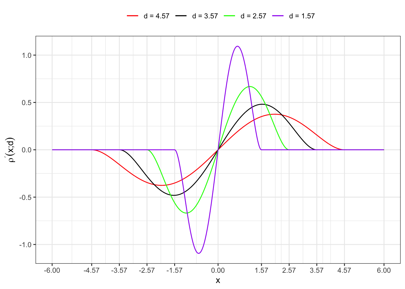
3.2 Second derivative
Plot code
ggplot()+
  geom_line(aes(grid, tukey_beaton_second(d[1])(grid), color = "p1"))+
  geom_line(aes(grid, tukey_beaton_second(d[2])(grid), color = "p2"))+
  geom_line(aes(grid, tukey_beaton_second(d[3])(grid), color = "p3"))+
  geom_line(aes(grid, tukey_beaton_second(d[4])(grid), color = "p4"))+
  scale_color_manual(values = c(p1 = "red", p2 = "black", p3 = "green", p4 = "purple"),
                     labels = c(p1 = paste0("d = ", d[1]),
                                p2 = paste0("d = ", d[2]),
                                p3 = paste0("d = ", d[3]),
                                p4 = paste0("d = ", d[4])))+
  theme_bw()+
  scale_x_continuous(breaks = c(min(grid),-d, 0, d, max(grid)))+
  theme(legend.position = "top")+
  labs(x = "x", y = TeX("$\\rho^{\\prime\\prime}(x; d)$"), color = NULL)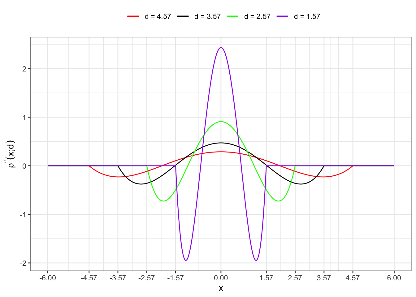
Citation
BibTeX citation:
@online{sartini2024,
  author = {Sartini, Beniamino},
  title = {Tukey Functions},
  date = {2024-05-01},
  url = {https://greenfin.it/statistics/robustness/tukey-functions.html},
  langid = {en}
}
For attribution, please cite this work as:
Sartini, Beniamino. 2024. “Tukey Functions.” May 1, 2024.
https://greenfin.it/statistics/robustness/tukey-functions.html.