Kumaraswamy distribution

In probability and statistics, the Kumaraswamy’s double bounded distribution is a family of continuous probability distributions defined on the interval \((0,1)\). It is similar to the Beta distribution, but much simpler to use especially in simulation studies since its probability density function, cumulative distribution function and quantile functions can be expressed in closed form. This distribution was originally proposed by Poondi Kumaraswamy. The distribution function is in Equation 1, the density function is in Equation 2, the quantile in Equation 3 and finally the random generator.
1 Distribution function
For \(x \in (0,1)\) and \(a > 0\), \(b > 0\) the distribution function is defined as:
\[ F(x; a, b) = 1 - (1-x^a)^{b} \tag{1}\]
In R code:
\[ \begin{aligned} \text{pkumaraswamy}({} & x, \; a = 1, \; b = 1, \\ & \text{log.p} = {\color{red}{\text{FALSE}}}, \\ & \text{lower.tail} = {\color{green}{\text{TRUE}}} \end{aligned} \]
Plot Kumaraswamy cdf
grid <- seq(0, 1, 0.01)
bind_rows(
  tibble(label = "a = 0.5, b = 0.5", a = 0.5, b = 0.5, x = grid, p = pkumaraswamy(x, a, b)),
  tibble(label = "a = 5, b = 1", a = 5, b = 1, x = grid, p = pkumaraswamy(x, a, b)),
  tibble(label = "a = 1, b = 3", a = 1, b = 3, x = grid, p = pkumaraswamy(x, a, b)),
  tibble(label = "a = 2, b = 2", a = 2, b = 2, x = grid, p = pkumaraswamy(x, a, b)),
  tibble(label = "a = 2, b = 5", a = 2, b = 5, x = grid, p = pkumaraswamy(x, a, b))
) %>%
  ggplot()+
  geom_line(aes(x, p, color = label))+
  theme_bw()+
  labs(x = TeX("$x$"), y = TeX("$F(x;a,b)$"), color = NULL)+
  theme(legend.position = "top")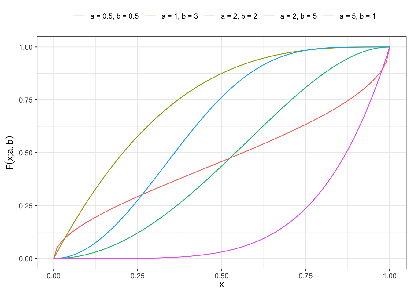
2 Density function
For \(x \in (0,1)\) and \(a > 0\), \(b > 0\) the density function is defined as:
\[ f(x; a, b) = abx^{a-1} (1-x^a)^{b-1} \tag{2}\]
In R code:
\[ \begin{aligned} \text{dkumaraswamy}({} & x, \; a = 1, \; b = 1, \\ & \text{log.p} = {\color{red}{\text{FALSE}}}) \end{aligned} \]
Plot pdf
grid <- seq(0.01, 0.99, 0.01)
bind_rows(
  tibble(label = "a = 0.5, b = 0.5", a = 0.5, b = 0.5, x = grid, p = dkumaraswamy(x, a, b)),
  tibble(label = "a = 5, b = 1", a = 5, b = 1, x = grid, p = dkumaraswamy(x, a, b)),
  tibble(label = "a = 1, b = 3", a = 1, b = 3, x = grid, p = dkumaraswamy(x, a, b)),
  tibble(label = "a = 2, b = 2", a = 2, b = 2, x = grid, p = dkumaraswamy(x, a, b)),
  tibble(label = "a = 2, b = 5", a = 2, b = 5, x = grid, p = dkumaraswamy(x, a, b))
) %>%
  ggplot()+
  geom_line(aes(x, p, color = label))+
  theme_bw()+
  labs(x = TeX("$x$"), y = TeX("$f(x;a,b)$"), color = NULL)+
  theme(legend.position = "top")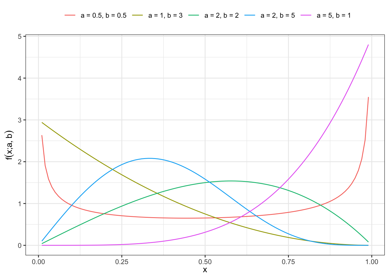
3 Quantile function
For \(p \in (0,1)\) and \(a > 0\), \(b > 0\) the quantile function is defined as:
\[ F^{-1}(p; a, b) = 1 - (1-p^{\frac{1}{b}})^{\frac{1}{a}} \tag{3}\]
In R code:
\[ \begin{aligned} \text{qkumaraswamy}({} & p, \; a = 1, \; b = 1, \\ & \text{log.p} = {\color{red}{\text{FALSE}}}, \\ & \text{lower.tail} = {\color{green}{\text{TRUE}}} \end{aligned} \]
4 Random generator
In general, given a random variable \(X \sim F_{X}\) following a certain distribution \(F_{X}\) and the correspondent quantile function \(F_{X}^{-1}\) (i.e. \(F_{X}^{-1}(F(X)) = X\)) it is possible to generate a random sample by simulating the grades. In steps:
Step 1.: simulate the grades \(u \sim \text{Unif}[0,1]\).
Step 2.: apply the quantile function of the desired distribution on the grades to obtain a simulations.
In R code:
\[ \text{rkumaraswamy}(n, \; a = 1, \; b = 1) \]
Plot pdf
params <- c(a = 1.5, b = 1.5)
x <- rkumaraswamy(5000, a = params[1], b = params[2])

ker <- density(x, from = min(x), to = max(x))
ker$pdf_th <- dkumaraswamy(ker$x, a = params[1], b = params[2])
#ker$pdf_th <- ker$pdf_th/sum(ker$pdf_th)
ker$pdf_emp <- ker$y#/sum(ker$y)

ggplot()+
  geom_line(aes(ker$x, ker$pdf_th), color = "red")+
  geom_line(aes(ker$x, ker$pdf_emp))+
  theme_bw()+
  labs(x = TeX("$x$"), y = TeX("$f(x;a,b)$"), color = NULL)+
  theme(legend.position = "top")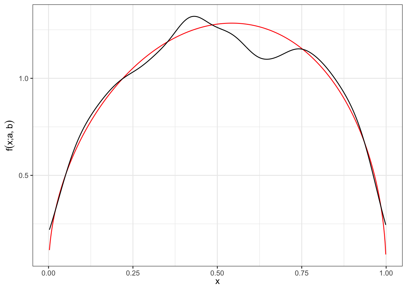
Citation
@online{sartini2024,
  author = {Sartini, Beniamino},
  title = {Kumaraswamy Distribution},
  date = {2024-05-01},
  url = {https://greenfin.it/statistics/distributions/kumaraswamy.html},
  langid = {en}
}