ARMA process

1 MA(q) process
In time series analysis, the moving-average process (MA) denotes a model for univariate time series. For a general order \(q\) it is defined as a process \(X_t \sim MA(q)\) when: \[ x_t = \mu + \sum_{i=1}^{q}\theta_i u_{t-i} + u_{t} \text{.} \] To be very general the error term is \(u_t \sim \text{MDS}(0,\sigma^2)\) is as ergotic \(\text{MDS}\), i.e. martingale difference sequence.
Let’s consider a process \(X_t \sim MA(1)\), i.e. \[ x_t = \mu + \theta_1 u_{t-1} + u_{t} \text{.} \] Independently from the distribution of \(u_t\), the long term expectation of the process is computed as \[ \mathbb{E}\{X_t\} = \mu + \mathbb{E}\{u_{t}\} + \theta_1 \mathbb{E}\{u_{t-1}\} = \mu \text{.} \] The variance instead, \[ \begin{aligned} \gamma_0 {} & = \mathbb{V}\{X_t\} = \\ & = \mathbb{V}\{u_{t}\} + \theta_1^2 \mathbb{V}\{u_{t-1}\} = \\ & = \sigma^2 + \theta_{1} \sigma^2 = \\ & = \sigma^2(1+\theta_{1}^2) \end{aligned} \] and, in general, the auto covariance function is defined as \[ \begin{aligned} \gamma_1 {} & = \mathbb{C}v\{X_t, X_{t-1}\} = \\ & = \mathbb{E}\{(u_{t} + \theta_{1}u_{t-1} )(u_{t-1} + \theta_{1}u_{t-2})\} = \\ & = \theta_{1} \mathbb{V}\{u_{t-1}\} = \\ & = \theta_{1} \sigma^2 \end{aligned} \] It follows that, the auto covariance function is bounded up to the first lag, i.e. \[ \begin{aligned} \sum_{j = 0}^{\infty} |\gamma_{j}| {} & = \gamma_{0} + \gamma_{1} + 0 + 0 + \dots = \\ & = \sigma^2 (1 + \theta_{1} + \theta_{1}^2) \end{aligned} \] Finally, the correlation between two lags is defined as: \[ \begin{aligned} \rho_{1} {} & = \mathbb{C}r\{X_t, X_{t-1}\} = \\ & = \frac{\mathbb{C}v\{X_t, X_{t-1}\}}{\sqrt{\mathbb{V}\{X_t\} \mathbb{V}\{X_{t-1}\}}} = \\ & = \frac{\gamma_1}{\gamma_0} = \frac{\theta_{1}}{1 + \theta_{1}^2} \text{.} \end{aligned} \] It follows that the process is always stationary independently from the parameter \(\theta_1\).
1.1 Example: MA(1)
Let’s simulate a moving-average Gaussian process \(X_t \sim MA(1)\), i.e. \[ x_t = \mu + \theta_1 u_{t-1} + u_{t} \text{,} \] where \(u_t \sim \mathcal{N}(0, \sigma^2)\).
MA(1) simulation
# ==================== Setups =====================
set.seed(1) # random seed
t_bar <- 2000 # number of simulations
par <- c(mu = 0, theta1 = 0.15) # parameters
sigma <- 1 # std. deviation residuals
lag.max <- 30 # maximum lag for ACF plot
Xt <- c(par[1]) # starting point
# ================== Simulation ===================
# Simulated residuals
eps <- rnorm(t_bar, mean=0, sd=sigma)
# Simulated MA(1)
for(t in 2:t_bar){
  Xt[t] <- par[1] + par[2]*eps[t-1] + eps[t]
}
# ===================== Plot ======================
# MA(1) simulation process
plot_ma <- ggplot()+
  geom_line(aes(1:t_bar, Xt), size = 0.2)+
  geom_line(aes(1:t_bar, par[1]), color = "red")+
  theme_bw()+
  labs(x = NULL, y = TeX("$X_t$"),
       subtitle = TeX(paste0("$\\mu:\\;", par[1],
                             "\\;\\; \\theta_{1}:\\;", par[2],
                             "\\;\\; \\sigma^2 : \\;", sigma^2,
                             "$")))
# MA(1) autocorrelation
lags <- 1:lag.max
x_breaks <- seq(1, lag.max, 2)
acf_j <- acf(Xt, plot = FALSE, lag.max = lag.max, type = "correlation")$acf[,,1][-1]
plot_acf <- ggplot()+
  geom_histogram(aes(lags, acf_j), stat = "identity",
                 color = "black", fill = "lightgray")+
  scale_x_continuous(breaks = x_breaks, labels = x_breaks)+
  labs(x = "Lag (i)", y = TeX("$\\rho{i}$"))+
  theme_bw()
gridExtra::grid.arrange(plot_ma, plot_acf, heights = c(0.6, 0.4))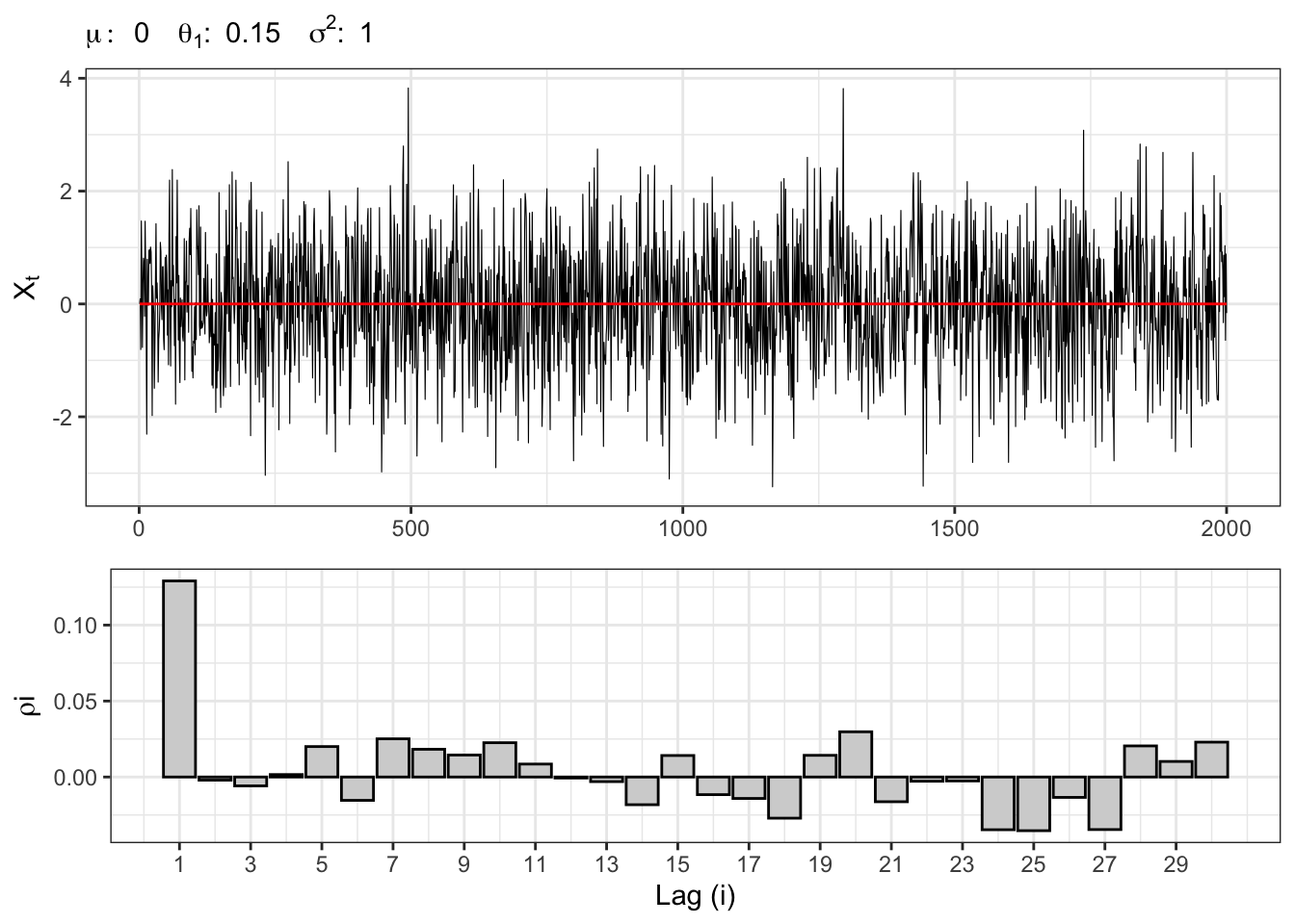
Table code
kab <- bind_rows(
     tibble(Statistic = "$$\\mathbb{E}\\{X_t\\}$$",
            Theoric = par[1],
            Empiric = mean(Xt)),
      tibble(Statistic = "$$\\mathbb{V}\\{X_t\\}$$",
             Theoric = sigma^2 * (1 + par[2]^2),
             Empiric = var(Xt)),
      tibble(Statistic = "$$\\mathbb{C}v\\{X_t, X_{t-1}\\}$$",
             Theoric = sigma^2 * par[2],
             Empiric = cov(Xt[-1], lag(Xt,1)[-1])),
     tibble(Statistic = "$$\\mathbb{C}r\\{X_t, X_{t-1}\\}$$",
            Theoric = par[2]/(1 + par[2]^2),
            Empiric = acf_j[1]))
kab %>%
  knitr::kable(format = "html", escape = FALSE, booktabs = FALSE, align = 'c') %>%
kableExtra::row_spec(0, color = "white", background = "green") | Statistic | Theoric | Empiric |
|---|---|---|
| $$\mathbb{E}\{X_t\}$$ | 0.0000000 | -0.0157117 |
| $$\mathbb{V}\{X_t\}$$ | 1.0225000 | 1.0937676 |
| $$\mathbb{C}v\{X_t, X_{t-1}\}$$ | 0.1500000 | 0.1412342 |
| $$\mathbb{C}r\{X_t, X_{t-1}\}$$ | 0.1466993 | 0.1290617 |
2 AR(p) process
Let’s consider an autoregressive process of order \(p\), namely \(X_t \sim AR(P)\), i.e. \[ x_t = \mu + \sum_{i=1}^{p}\phi_{i} x_{t-i} + u_{t} \text{,} \] where in general \(u_t \sim \text{MDS}(0, \sigma^2)\).
Let’s consider a process \(X_t \sim AR(1)\), i.e. \[ x_t = \mu + \phi_{1} x_{t-1} + u_{t} \text{.} \] Through recursion up to time 0 it is possible to express an AR(1) model as an MA(\(\infty\)), i.e. \[ X_t = \phi_1^{t} X_0 + \mu \sum_{i=0}^{t-1} \phi_{1}^{i} + \sum_{i = 0}^{t-1} \phi_{1}^{i} u_{t-i} \] where the process is stationary if and only if \(|\phi_1|<1\). In fact, independently from the specific distribution of the residuals \(u_t\), the unconditional expectation of an AR(1) converges if and only if \(|\phi_1|<1\), i.e. \[ \mathbb{E}\{X_t\} = \phi_1^{t} X_0 + \mu \sum_{i=0}^{t-1} \phi_{1}^{i} = \frac{\mu}{1-\phi_1} \]
The variance instead is computed as: \[ \gamma_0 = \mathbb{V}\{X_t\} = \sum_{i=0}^{t-1} \phi_{1}^{2i} \sigma^{2} = \frac{\sigma^{2}}{1-\phi_{1}^2} \] The auto covariance decays exponentially fast depending on the parameter \(\phi_1\), i.e. \[ \begin{aligned} \gamma_1 {} & = \mathbb{C}v\{X_t, X_{t-1}\} = \phi_{1} \frac{\sigma^{2}}{1-\phi_{1}^2} = \phi_1 \gamma_0 \end{aligned} \] and in general: \[ \begin{aligned} \gamma_k {} & = \mathbb{C}v\{X_t, X_{t-k}\} = \phi_{1}^{|k|} \gamma_0 \text{.} \end{aligned} \] Finally, the auto correlation function is given by: \[ \begin{aligned} \rho_{1} {} & = \mathbb{C}r\{X_t, X_{t-1}\} = \\ & = \frac{\mathbb{C}v\{X_t, X_{t-1}\}}{\sqrt{\mathbb{V}\{X_t\} \mathbb{V}\{X_{t-1}\}}} = \\ & = \frac{\gamma_1}{\gamma_0} = \phi_1 \end{aligned} \] and in general: \[ \begin{aligned} \rho_{k} {} & = \mathbb{C}r\{X_t, X_{t-k}\} = \phi_{1}^{|k|} \text{.} \end{aligned} \]
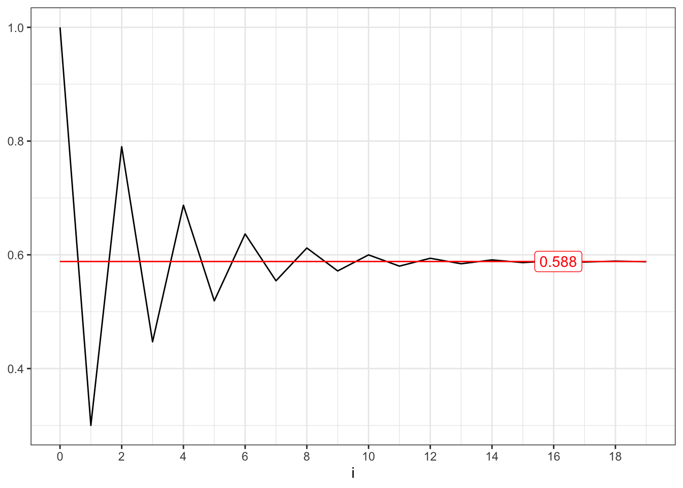
The stationary of an AR(1) process is related to the convergence of two series. The unconditional expectation converges if and only if following series converges, i.e. \[ \sum_{i=0}^{\infty} \phi_1^{i} = \frac{1}{1-\phi_1} \quad\text{iff}\quad |\phi_1| < 1 \text{.} \]
Convergent series (I)
# ==================== Setups =====================
phi <- c(0.7, -0.7)
min_i <- 0
max_i <- 20
i <- seq(min_i, max_i - 1, 1)
y_breaks <- seq(min_i, max_i, 2)
x_labels <- quantile(i, 0.85)
# =================================================
# Convergent series 0 < phi < 1
series1 <- cumsum(phi[1]^i)
limit1 <- 1/(1 - phi[1])
plot_1 <- ggplot()+
  geom_line(aes(i, series1))+
  geom_line(aes(i, limit1), color = "red")+
  geom_label(aes(x_labels, limit1, label = round(limit1, 3)), color = "red")+
  labs(x = "i", y = TeX("$\\sum_{i=0}^{\\infty} \\phi_{1}^{i}$"))+
  scale_x_continuous(breaks = y_breaks)+
  theme_bw()
# Convergent series -1 < phi < 0
series2 <- cumsum(phi[2]^i)
limit2 <- 1/(1 - phi[2])
plot_2 <- ggplot()+
  geom_line(aes(i, series2))+
  geom_line(aes(i, limit2), color = "red")+
  geom_label(aes(x_labels, limit2, label = round(limit2, 3)), color = "red")+
  labs(x = "i", y = NULL)+
  scale_x_continuous(breaks = y_breaks)+
  theme_bw()
plot_1
plot_2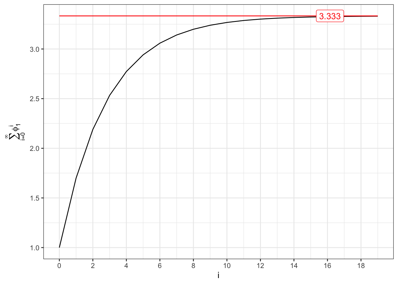
The convergence of the variance is related to the following series, i.e. \[ \sum_{i=0}^{\infty} \phi_1^{2i} = \frac{1}{1-\phi_1^2} \quad\text{iff}\quad |\phi_1| < 1 \text{.} \]
Convergent series (II)
# Convergent series |phi| < 1
series1 <- cumsum(phi[1]^(i*2))
limit1 <- 1/(1 - phi[1]^2)
ggplot()+
  geom_line(aes(i, series1))+
  geom_line(aes(i, limit1), color = "red")+
  geom_label(aes(x_labels, limit1, label = round(limit1, 3)), color = "red")+
  labs(x = "i", y = TeX("$\\sum_{i=0}^{\\infty} \\phi_{1}^{2i}$"), subtitle = TeX("$|\\phi_1| < 1$"))+
  scale_x_continuous(breaks = y_breaks)+
  theme_bw()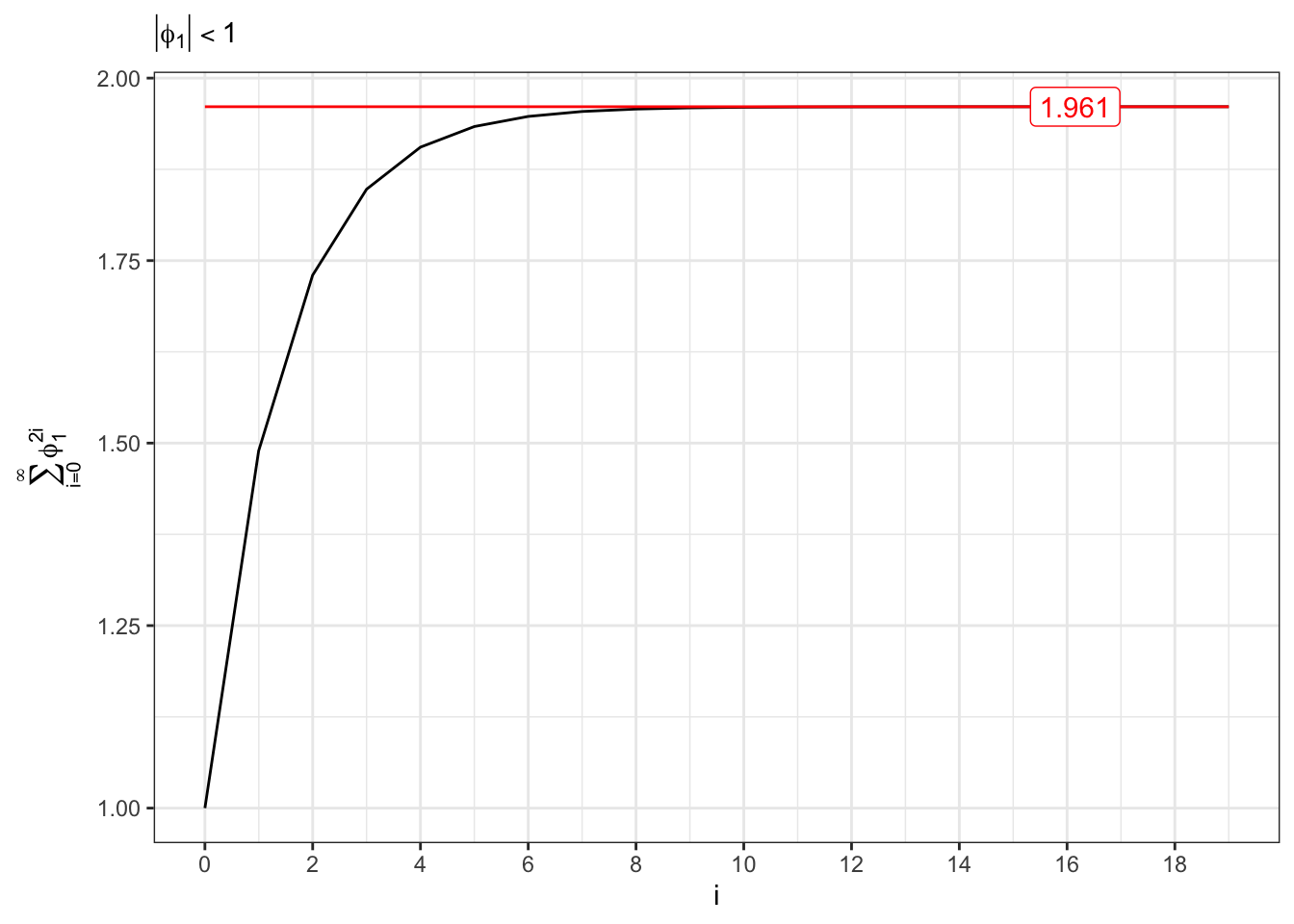
2.1 Example: AR(1)
Let’s simulate an autoregressive Gaussian process, namely \(X_t \sim AR(1)\), i.e. \[ x_t = \mu + \phi_{1} x_{t-1} + u_{t} \text{,} \] where \(u_t \sim \mathcal{N}(0, \sigma^2)\).
AR(1) simulation
# ==================== Setups =====================
set.seed(2) # random seed
t_bar <- 5000 # number of simulations
par <- c(mu = 0.5, phi1 = 0.95) # parameters
sigma <- 1 # sd of epsilon
lag.max <- 30 # maximum lag for acf
Xt <- c(par[1]/(1-par[2])) # initial point
# ================== Simulation ===================
# Simulated residuals
eps <- rnorm(t_bar, mean=0, sd=sigma)
# simulated AR(1)
for(t in 2:t_bar){
  Xt[t] <- par[1] + par[2]*Xt[t-1] + eps[t]
}
# ===================== Plot ======================
# AR(1) simulation
plot_ar <- ggplot()+
  geom_line(aes(1:t_bar, Xt), size = 0.2)+
  geom_line(aes(1:t_bar, par[1]/(1-par[2])), color = "red")+
  theme_bw()+
  labs(x = "t", y = TeX("$X_t$"),
       subtitle = TeX(paste0("$\\mu:\\;", par[1],
                             "\\;\\; \\phi_{1}:\\;", par[2],
                             "\\;\\; \\sigma^2 : \\;", sigma^2,
                             "$")))
# AR(1) autocorrelation
lags <- 1:lag.max
x_breaks <- seq(1, lag.max, 2)
acf_j <- acf(Xt, plot = FALSE, lag.max = lag.max, type = "cov")$acf[,,1][-1]
plot_acf <- ggplot()+
  geom_histogram(aes(lags, acf_j), stat = "identity", fill = "lightgray", color = "black")+
  geom_line(aes(lags, (par[2]^abs(lags))*(sigma^2)/(1-par[2]^2) ), color = "blue")+
  scale_x_continuous(breaks = x_breaks, labels = x_breaks)+
  theme_bw() +
  labs(x = "Lag (i)", y = TeX("$\\gamma_{i}$"),
       subtitle = "Exponential decay autocovariance")
gridExtra::grid.arrange(plot_ar, plot_acf, heights = c(0.6, 0.4))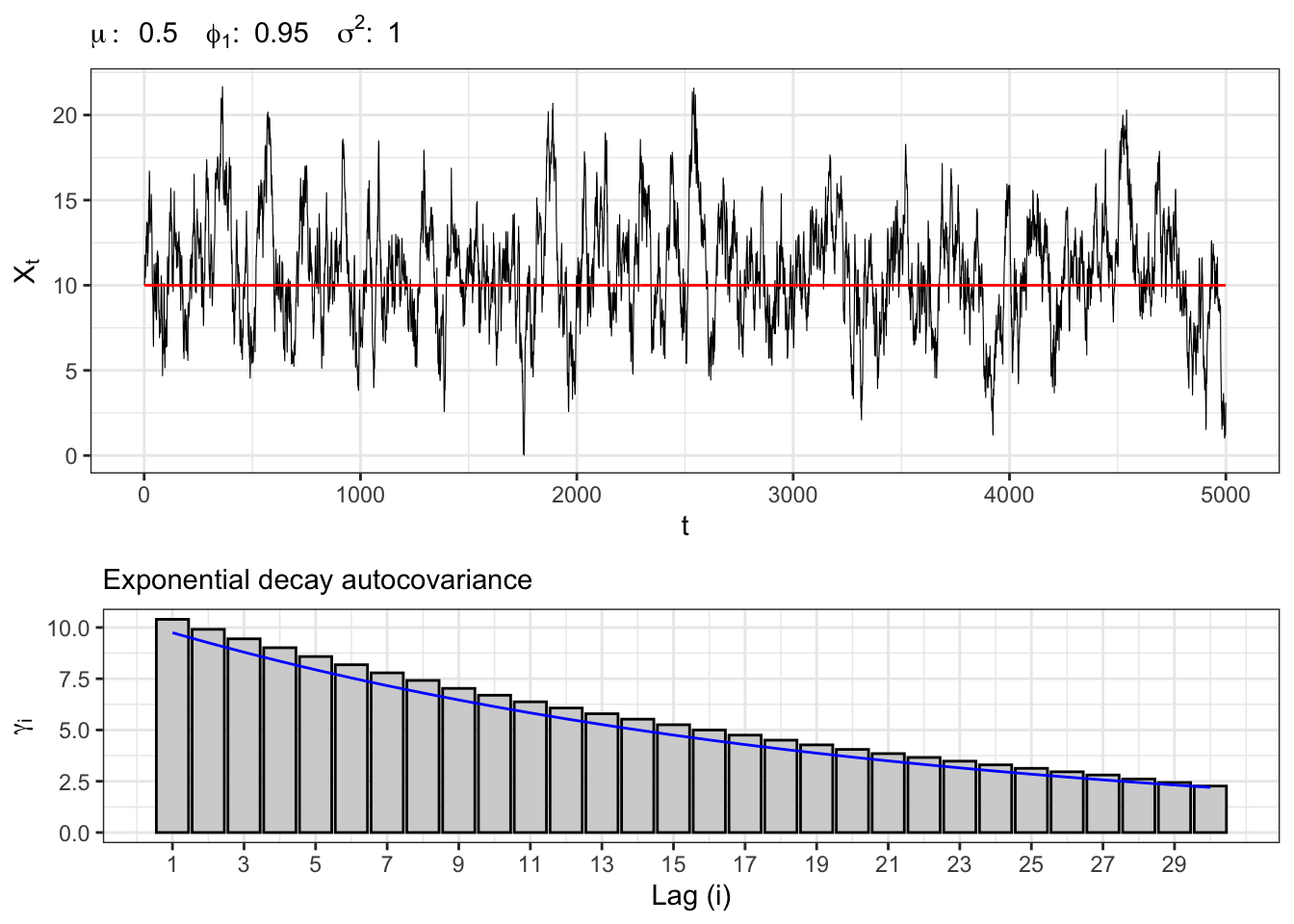
2.2 Example: stationary AR(1)
Stationary AR(1)
# ==================== Setups =====================
set.seed(3) # random seed
t_bar <- 120 # number of steps ahead
j_bar <- 1000 # number of simulations
sigma <- 1 # standard deviation of epsilon
par <- c(mu = 0, phi1 = 0.7) # parameters
X0 <- par[1]/(1-par[2]) # initial point
t_sample <- c(30,60,90) # sample times
# ================== Simulation ===================
# Process Simulations
scenarios <- tibble()
for(j in 1:j_bar){
  Xt <- c(X0)
  # Simulated residuals
  eps <- rnorm(t_bar, 0, sigma)
  # Simulated AR(1)
  for(t in 2:t_bar){
    Xt[t] <- par[1] + par[2]*Xt[t-1] + eps[t]
  }
  df <- tibble(j = rep(j, t_bar), t = 1:t_bar, Xt = Xt, eps = eps)
  scenarios <- bind_rows(scenarios, df)
}
# ===================== Plot ======================
# Trajectory j
df_j <- dplyr::filter(scenarios, j == 6)
# Sample at different times
df_t1 <- dplyr::filter(scenarios, t == t_sample[1])
df_t2 <- dplyr::filter(scenarios, t == t_sample[2])
df_t3 <- dplyr::filter(scenarios, t == t_sample[3])
# Paths plots
ggplot()+
  geom_line(data = scenarios, aes(t, Xt, group = j), alpha = 0.2, size = 0.2)+
  geom_line(data = df_j, aes(t, par[1]/(1-par[2])), color = "red")+
  geom_line(data = df_j, aes(t, Xt), color = "green", size = 0.4)+
  geom_point(data = df_t1, aes(t, Xt), color = "magenta", size = 0.1)+
  geom_point(data = df_t2, aes(t, Xt), color = "magenta", size = 0.1)+
  geom_point(data = df_t3, aes(t, Xt), color = "magenta", size = 0.1)+
  scale_x_continuous(breaks = seq(0, 100, 30))+
  theme_bw()+
  labs(x = "t", y = TeX("$X_t$"),
       subtitle = TeX(paste0("$\\mu:\\;", par[1],
                             "\\;\\; \\phi_{1}:\\;", par[2],
                             "\\;\\; \\sigma^2 : \\;", sigma^2,
                             "$")))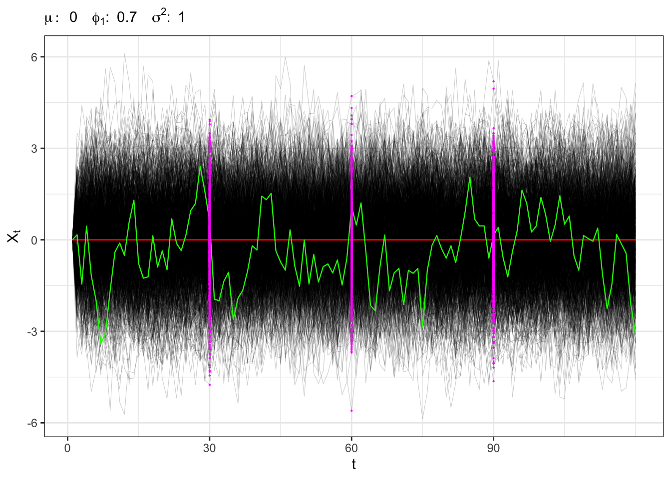
Sampling the process for different \(t\) we expect that, on a large number of simulations, the distribution will be normal with stationary moments, i.e. \[ X_t \sim \mathcal{N}\left(\frac{\mu}{1-\phi_{1}}, \frac{\sigma^{2}}{1-\phi_{1}^2} \right) \forall t \text{.} \]
Sampled AR(1)
# ================== Setups ==================
bins <- 30 # bins for histograms
# Stationary moments
e_x <- par[1]/(1-par[2])
sd_x <- sqrt((sigma^2)/(1 - par[2]^2))
# ================= Sample 1 =================
samp1 <- df_t1
df_grid1 <- list()
# Grid of points
df_grid1$grid <- seq(min(samp1$Xt), max(samp1$Xt), length.out = nrow(samp1))
# Stationary theoric pdf
df_grid1$pdf_theoric <- dnorm(df_grid1$grid, e_x, sd_x)
# Stationary empiric pdf
df_grid1$pdf_empiric <- dnorm(df_grid1$grid, mean(samp1$Xt), sd(samp1$Xt))
df_grid1 <- bind_cols(df_grid1)
plot_t1 <- ggplot()+
  geom_histogram(data = samp1, aes(Xt, after_stat(density)),
                 bins = bins, color = "black", fill = "lightgray")+
  geom_line(data = df_grid1, aes(grid, pdf_theoric), color = "magenta")+
  geom_line(data = df_grid1, aes(grid, pdf_empiric), color = "blue")+
  labs(subtitle = paste0("t = ", samp1$t[1]), x = NULL, y = NULL)+
  theme_bw()
# ================= Sample 2 =================
samp2 <- df_t2
df_grid2 <- list()
# Grid of points
df_grid2$grid <- seq(min(samp2$Xt), max(samp2$Xt), length.out = nrow(samp2))
# Stationary theoric pdf
df_grid2$pdf_theoric <- dnorm(df_grid2$grid, e_x, sd_x)
# Stationary empiric pdf
df_grid2$pdf_empiric <- dnorm(df_grid2$grid, mean(samp2$Xt), sd(samp2$Xt))
df_grid2 <- bind_cols(df_grid2)
plot_t2 <- ggplot()+
  geom_histogram(data = samp2, aes(Xt, after_stat(density)),
                 bins = bins, color = "black", fill = "lightgray")+
  geom_line(data = df_grid2, aes(grid, pdf_theoric), color = "magenta")+
  geom_line(data = df_grid2, aes(grid, pdf_empiric), color = "blue")+
  labs(subtitle = paste0("t = ", samp2$t[1]), x = NULL, y = NULL)+
  theme_bw()
# ================= Sample 3 =================
samp3 <- df_t3
df_grid3 <- list()
# Grid of points
df_grid3$grid <- seq(min(samp3$Xt), max(samp3$Xt), length.out = nrow(samp3))
# Stationary theoric pdf
df_grid3$pdf_theoric <- dnorm(df_grid3$grid, e_x, sd_x)
# Stationary empiric pdf
df_grid3$pdf_empiric <- dnorm(df_grid3$grid, mean(samp3$Xt), sd(samp3$Xt))
df_grid3 <- bind_cols(df_grid3)
plot_t3 <- ggplot()+
  geom_histogram(data = samp3, aes(Xt, after_stat(density)),
                 bins = bins, color = "black", fill = "lightgray")+
  geom_line(data = df_grid3, aes(grid, pdf_theoric), color = "magenta")+
  geom_line(data = df_grid3, aes(grid, pdf_empiric), color = "blue")+
  labs(subtitle = paste0("t = ", samp3$t[1]), x = NULL, y = NULL)+
  theme_bw()
gridExtra::grid.arrange(plot_t1, plot_t2, plot_t3, ncol = 3)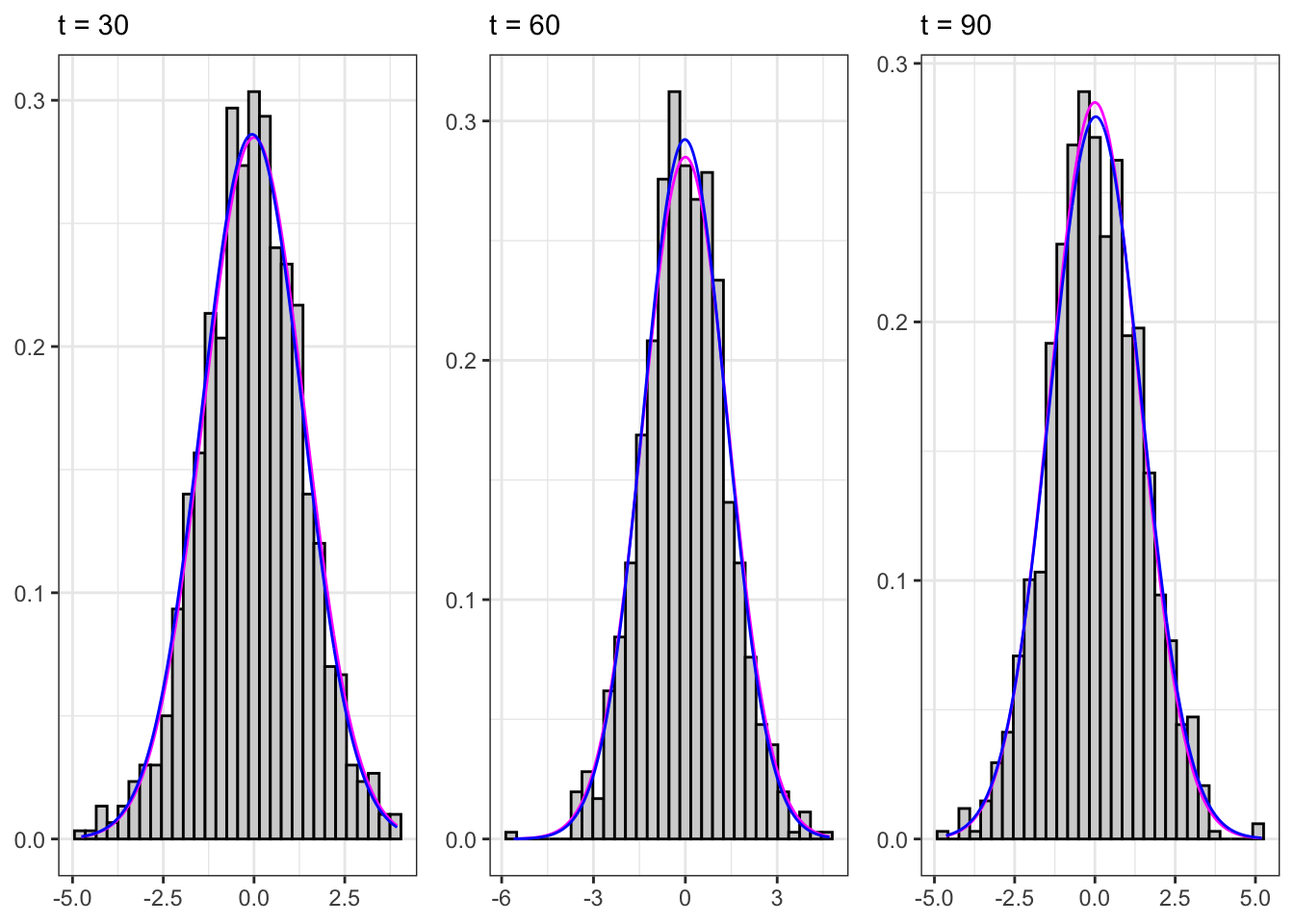
| Statistic | Theoric | Empiric |
|---|---|---|
| $$\mathbb{E}\{X_t\}$$ | 0.000000 | -0.0027287 |
| $$\mathbb{V}\{X_t\}$$ | 1.960784 | 1.9530614 |
| $$\mathbb{C}v\{X_{t}, X_{t-1}\}$$ | 1.372549 | 1.3586670 |
| $$\mathbb{C}r\{X_{t}, X_{t-1}\}$$ | 0.700000 | 0.6956660 |
2.3 Example: non-stationary AR(1)
A non-stationary process has \(\phi_1 = 1\), for example let’s consider a random walk with drift, i.e. \[ x_t = \mu + x_{t-1} + u_{t} \text{,} \] or equivalently \[ x_t = X_0 + \mu t + \sum_{i = 0}^{t-1} u_{t-i} \text{.} \] In this setting, the expectation and variance of the process do not converges but tends to explode as \(t\) increases, i.e. \[ \begin{aligned} {} & \mathbb{E}\{X_t\} = X_0 + \mu t \\ & \mathbb{V}\{X_t\} = t \sigma^{2} \end{aligned} \quad\text{iff}\quad \phi_1 = 1 \]
Non-stationary AR(1)
# ==================== Setups =====================
set.seed(5) # random seed
t_bar <- 120 # number of steps ahead
j_bar <- 1000 # number of simulations
sigma0 <- 1 # standard deviation of epsilon
par <- c(mu = 0.3, phi1 = 1) # parameters
X0 <- c(0) # initial point
t_sample <- c(30,60,90) # sample times
# ================== Simulation ===================
# Process Simulations
scenarios <- tibble()
for(j in 1:j_bar){
  # Initialize X0 and variance
  Xt <- rep(X0, t_bar)
  sigma <- rep(sigma0, t_bar)
  # Simulated residuals
  eps <- rnorm(t_bar, mean=0, sd=sigma0)
  for(t in 2:t_bar){
    sigma[t] <- sigma0*sqrt(t)
    Xt[t] <- par[1] + par[2]*Xt[t-1] + eps[t]
  }
  df <- tibble(j = rep(j, t_bar), t = 1:t_bar, Xt = Xt,
               sigma = sigma, eps = eps)
  scenarios <- dplyr::bind_rows(scenarios, df)
}
# Compute simulated moments
scenarios <- scenarios %>%
  group_by(t) %>%
  mutate(e_x = mean(Xt), sd_x = sd(Xt))

# ===================== Plot ======================
# Trajectory j
df_j <- dplyr::filter(scenarios, j == 6)
# Sample at different times
df_t1 <- dplyr::filter(scenarios, t == t_sample[1])
df_t2 <- dplyr::filter(scenarios, t == t_sample[2])
df_t3 <- dplyr::filter(scenarios, t == t_sample[3])
# Non-stationary paths
plot_paths <- ggplot()+
  geom_line(data = scenarios, aes(t, Xt, group = j),
            alpha = 0.5, size = 0.1)+
  geom_line(data = df_j, aes(t, e_x, group = j), color = "red")+
  geom_line(data = df_j, aes(t, Xt), color = "green", size = 0.4)+
  geom_point(data = df_t1, aes(t, Xt), color = "magenta", size = 0.1)+
  geom_point(data = df_t2, aes(t, Xt), color = "magenta", size = 0.1)+
  geom_point(data = df_t3, aes(t, Xt), color = "magenta", size = 0.1)+
  scale_x_continuous(breaks = seq(0, 100, 30))+
  theme_bw()+
  labs(x = NULL, y = TeX("$X_t$"),
       subtitle = TeX(paste0("$\\mu:\\;", par[1],
                             "\\;\\; \\phi_{1}:\\;", par[2],
                             "\\;\\; \\sigma^2 : \\;", sigma0^2,
                             "$")))
# Non-stationary std. deviation
plot_sigma <- ggplot(df_j)+
  geom_line(aes(t, sigma, group = j), alpha = 1)+
  geom_line(aes(t, sd_x, group = j), alpha = 1, color = "blue")+
  labs(x = "t", y = TeX("$\\sigma_{t}$"))+
  theme_bw()
gridExtra::grid.arrange(plot_paths, plot_sigma, heights = c(0.7, 0.3))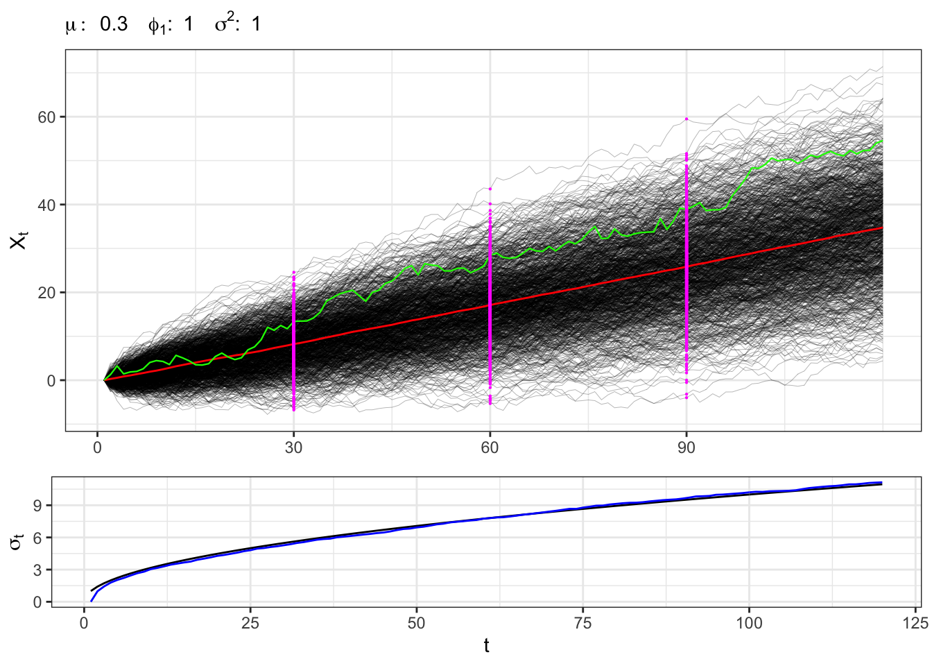
Sampling the process for different \(t\) we expect that, on a large number of simulations, the distribution will be normal with non-stationary moments, i.e. \[ X_t \sim \mathcal{N}\left(\mu t, \sigma^{2} t \right) \text{.} \]
Sampled non-stationary AR(1)
# ================== Setups ==================
bins <- 30 # bins for histograms
# ================= Sample 1 =================
samp1 <- df_t1
df_grid1 <- list()
# Grid of points
df_grid1$grid <- seq(min(samp1$Xt), max(samp1$Xt), length.out = nrow(samp1))
# Non stationary theoric pdf
df_grid1$pdf_theoric <- dnorm(df_grid1$grid, X0 + par[1]*samp1$t[1], samp1$sigma[1])
# Non stationary empiric pdf
df_grid1$pdf_empiric <- dnorm(df_grid1$grid, samp1$e_x[1], samp1$sd_x[1])
df_grid1 <- bind_cols(df_grid1)
plot_t1 <- ggplot()+
  geom_histogram(data = samp1, aes(Xt, after_stat(density)),
                 bins = bins, color = "black", fill = "lightgray")+
  geom_line(data = df_grid1, aes(grid, pdf_theoric), color = "magenta")+
  geom_line(data = df_grid1, aes(grid, pdf_empiric), color = "blue")+
  labs(subtitle = paste0("t = ", samp1$t[1]), x = NULL, y = NULL)+
  theme_bw()
# ================= Sample 2 =================
samp2 <- df_t2
df_grid2 <- list()
# Grid of points
df_grid2$grid <- seq(min(samp2$Xt), max(samp2$Xt), length.out = nrow(samp2))
# Non stationary theoric pdf
df_grid2$pdf_theoric <- dnorm(df_grid2$grid, X0 + par[1]*samp2$t[1], samp2$sigma[1])
# Non stationary empiric pdf
df_grid2$pdf_empiric <- dnorm(df_grid2$grid, samp2$e_x[1], samp2$sd_x[1])
df_grid2 <- bind_cols(df_grid2)
plot_t2 <- ggplot()+
  geom_histogram(data = samp2, aes(Xt, after_stat(density)),
                 bins = bins, color = "black", fill = "lightgray")+
  geom_line(data = df_grid2, aes(grid, pdf_theoric), color = "magenta")+
  geom_line(data = df_grid2, aes(grid, pdf_empiric), color = "blue")+
  labs(subtitle = paste0("t = ", samp2$t[1]), x = NULL, y = NULL)+
  theme_bw()
# ================= Sample 3 =================
samp3 <- df_t3
df_grid3 <- list()
# Grid of points
df_grid3$grid <- seq(min(samp3$Xt), max(samp3$Xt), length.out = nrow(samp3))
# Non stationary theoric pdf
df_grid3$pdf_theoric <- dnorm(df_grid3$grid, X0 + par[1]*samp3$t[1], samp3$sigma[1])
# Non stationary empiric pdf
df_grid3$pdf_empiric <- dnorm(df_grid3$grid, samp3$e_x[1], samp3$sd_x[1])
df_grid3 <- bind_cols(df_grid3)
plot_t3 <- ggplot()+
  geom_histogram(data = samp3, aes(Xt, after_stat(density)),
                 bins = bins, color = "black", fill = "lightgray")+
  geom_line(data = df_grid3, aes(grid, pdf_theoric), color = "magenta")+
  geom_line(data = df_grid3, aes(grid, pdf_empiric), color = "blue")+
  labs(subtitle = paste0("t = ", samp3$t[1]), x = NULL, y = NULL)+
  theme_bw()
gridExtra::grid.arrange(plot_t1, plot_t2, plot_t3, ncol = 3)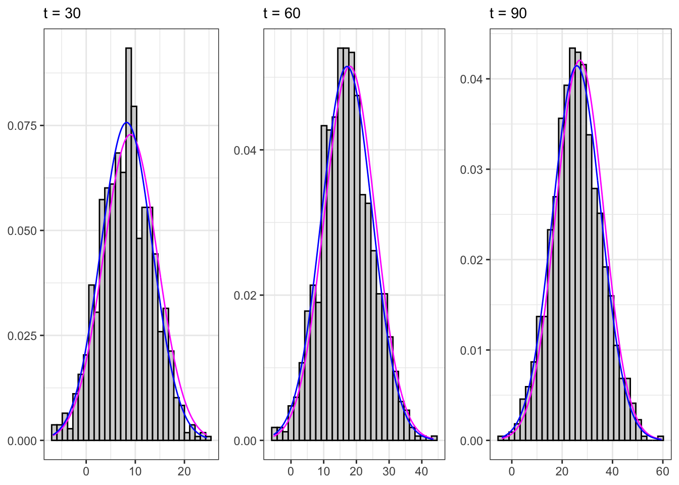
3 ARMA(p,q) process
An ARMA(p,q) process is a combination of an MA(q) and an AR(p) processes, i.e. an \(X_t \sim ARMA(p,q)\) is defined as \[ x_t = \mu + \sum_{i=1}^{p}\phi_{i} x_{t-i} + \sum_{j=1}^{q}\theta_{j} u_{t-j} + u_{t} \text{,} \] where in general \(u_t \sim \text{MDS}(0, \sigma^2)\).
3.1 Example: ARMA(1,1)
Let’s simulate a Gaussian autoregressive moving-average process, namely \(X_t \sim ARMA(1,1)\), i.e. \[ x_t = \mu + \phi_{1} x_{t-1} + \theta_{1} u_{t-1} + u_{t} \text{,} \] where \(u_t \sim \mathcal{N}(0, \sigma^2)\).
ARMA(1,1) simulation
# ======================== Setups ========================
set.seed(6) # random seed
t_bar <- 2000 # Number of steps ahead
# Parameters
par <- c(mu = 0.5, phi1 = 0.95, theta1 = 0.45)
sigma <- 1 # Standard deviation of epsilon
lag.max <- 30 # Maximum lag for acf
# ===================== Simulations =====================
# Initial value
Xt <- c(par[1]/(1-par[2]))
# Simulated residuals
eps <- rnorm(t_bar, 0, sigma)
# Simulated ARMA(1,1)
for(t in 2:t_bar){
  Xt[t] <- par[1] + par[2]*Xt[t-1] + par[3]*eps[t-1] + eps[t]
}
# ======================== Plot =========================
# ARMA(1,1) simulation
plot_arma <- ggplot()+
  geom_line(aes(1:t_bar, Xt), size = 0.2)+
  theme_bw()+
  labs(x = "t", y = TeX("$X_t$"),
       subtitle = TeX(paste0("$\\mu:\\;", par[1],
                             "\\;\\; \\phi_{1}:\\;", par[2],
                             "\\;\\; \\theta_{1}:\\;", par[3],
                             "\\;\\; \\sigma^2 : \\;", sigma^2,
                             "$")))
# ARMA(1,1) autocorrelation
lags <- 1:lag.max
y_breaks <- seq(1, lag.max, 2)
acf_j <- acf(Xt, plot = FALSE, lag.max = lag.max, type = "cor")$acf[,,1][-1]
plot_acf <- ggplot()+
  geom_histogram(aes(lags, acf_j), stat = "identity", fill = "gray", color = "black")+
  scale_x_continuous(breaks = y_breaks)+
  theme_bw()+
  labs(x = "Lag (i)", y = TeX("$\\rho_{i}$"),
       subtitle = "Exponential decay autocorrelation")
gridExtra::grid.arrange(plot_arma, plot_acf, heights = c(0.6, 0.4))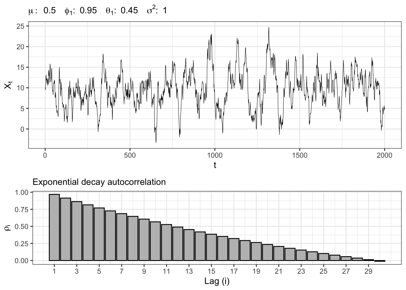
3.2 Example: ARMA(2,3)
Let’s simulate another Gaussian autoregressive moving-average process, namely \(X_t \sim ARMA(2,3)\), i.e. \[ x_t = \mu + \sum_{i = 1}^{2} \phi_{i} x_{t-i} + \sum_{j = 1}^{3} \theta_{j} u_{t-j} + u_{t} \text{,} \] where \(u_t \sim \mathcal{N}(0, \sigma^2)\).
ARMA(2,3) simulation
# ======================== Setups ========================
set.seed(7) # random seed
t_bar <- 4000 # Number of steps ahead
# Parameters
par <- c(mu = 0, phi1 = 0.45, phi2 = 0.25,
         theta1 = 0.55, theta1 = 0.35, theta1 = 0.15)
sigma <- 1 # Standard deviation of epsilon
lag.max <- 30 # Maximum lag for acf
# ===================== Simulations =====================
# Random seed
set.seed(1)
# Initial value
Xt <- rep(0, 4)
# Simulated ARMA(1,1)
eps <- rnorm(t_bar, 0, sigma)
for(t in 4:t_bar){
  # AR component
  Xt[t] <- par[1] + par[2]*Xt[t-1] + par[3]*Xt[t-2]
  # MA component
  Xt[t] <- Xt[t] + par[4]*eps[t-1] + par[5]*eps[t-2] + par[6]*eps[t-3] + eps[t]
}
# ======================== Plot =========================
# ARMA(1,1) simulation
plot_arma <- ggplot()+
  geom_line(aes(1:t_bar, Xt), size = 0.2)+
  theme_bw()+
  labs(x = "t", y = TeX("$X_t$"),
       subtitle = TeX(paste0("$\\mu:\\;", par[1],
                             "\\;\\; \\phi_{1}:\\;", par[2],
                             "\\;\\; \\theta_{1}:\\;", par[3],
                             "\\;\\; \\theta_{2}:\\;", par[4],
                             "\\;\\; \\theta_{3}:\\;", par[5],
                             "\\;\\; \\sigma^2 : \\;", sigma^2,
                             "$")))
# ARMA(1,1) autocorrelation
lags <- 1:lag.max
y_breaks <- seq(1, lag.max, 2)
acf_j <- acf(Xt, plot = FALSE, lag.max = lag.max, type = "cor")$acf[,,1][-1]
plot_acf <- ggplot()+
  geom_histogram(aes(lags, acf_j), stat = "identity", fill = "gray", color = "black")+
  scale_x_continuous(breaks = y_breaks)+
  theme_bw()+
  labs(x = "Lag (i)", y = TeX("$\\rho_{i}$"),
       subtitle = "Exponential decay autocorrelation")
gridExtra::grid.arrange(plot_arma, plot_acf, heights = c(0.6, 0.4))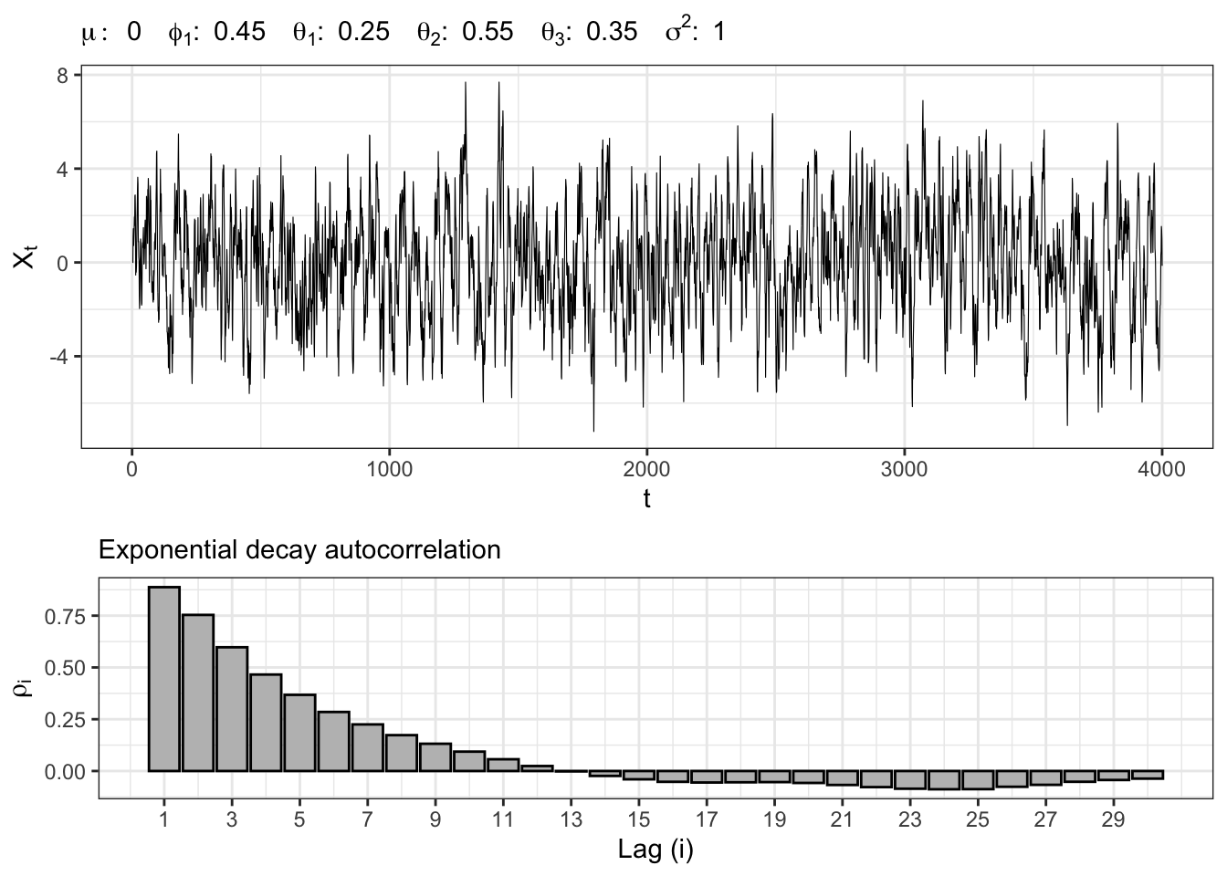
Citation
@online{sartini2024,
  author = {Sartini, Beniamino},
  title = {ARMA Process},
  date = {2024-05-01},
  url = {https://greenfin.it/statistics/arma-models.html},
  langid = {en}
}