ARCH-GARCH process

1 ARCH(p) process
The autoregressive conditional heteroskedasticity (ARCH) models were introduced in 1982 by Robert Engle to model varying (conditional) variance of time series. It is often found in economics that the larger values of time series also lead to larger instability. Let’s define a time series such as \(X_t \sim ARCH(p)\), then it is defined as: \[ \begin{aligned} & {} x_t = \mu + e_t \\ & e_t = \sigma_t u_t \\ & \sigma_t^{2} = \omega + \sum_{i=1}^{p} \alpha_i e_{t-i}^2 \end{aligned} \] where \(u_t \sim \text{MDS}(0,1)\).
The unconditional and conditional mean of a process \(X_t \sim ARCH(p)\) are equal to: \[ \mathbb{E}\{X_t\} = \mathbb{E}\{X_t|I_{t-1}\} = \mu \text{,} \] where \(I_{t-1}\) denotes the information available up to time \(t-1\). Instead, the long term variance of the process, i.e. the unconditional variance, is defined as: \[ \begin{aligned} \mathbb{V}\{X_t\} {} & = \mathbb{V}\{\mu + \sigma_t u_t\} = {} & \\ & = \mathbb{V}\{\sigma_t u_t\} = & (\mathbb{E}\{u_t\} = 0) \\ & = \mathbb{E}\{\sigma_t^2 u_t^2\} = & (u_t \text{ iid}) \\ & = \mathbb{E}\{\sigma_t^2\} \mathbb{E}\{u_t^2\} = & (\mathbb{E}\{u_t^2\} = 1) \\ & = \mathbb{E}\{\sigma_t^2\} \cdot 1 \end{aligned} \] where the unconditional expectation of the stochastic variance is given by \[ \mathbb{E}\{\sigma_t^2\} = \frac{\omega}{1 - \sum_{i=1}^{p} \alpha_i} \text{.} \] It is clear that, in general \(\omega \neq 0\) and, to ensure that the process is stationary, the following condition on the parameters must be satisfied: \[ \sum_{i=1}^{p} \alpha_i < 1 \quad \alpha_i > 0 \;\; \forall i \]
1.1 Example: ARCH(1) process
Let’s simulate an ARCH(1) process with normal residuals, namely \(X_t \sim ARCH(1)\), i.e. \[ \begin{aligned} & {} x_t = \mu + e_t \\ & e_t = \sigma_t u_t \\ & \sigma_t^{2} = \omega + \alpha_1 e_{t-1}^2 \end{aligned} \] where \(u_t \sim \mathcal{N}(0,1)\).
ARCH(1) simulation
# Random seed
set.seed(1)
# ==================== Setups =====================
# Nsumber of simulations
t_bar <- 500
# Parameters
par <- c(mu=0.5, omega=0.4, alpha1=0.25)
# Long-term std deviation of residuals
sigma_eps <- sqrt(par[2]/(1-par[3]))
# ================== Simulation ===================
# Initial point
Xt <- rep(par[1], 1)
# Store stochastic variance
sigma <- rep(sigma_eps, 1)
# Simulated residuals
eps <- rnorm(t_bar, 0, 1)
for(t in 2:t_bar){
  # ARCH(1) variance
  sigma[t] <- par[3]*eps[t-1]^2
  # ARCH(1) std. deviation
  sigma[t] <- sqrt(par[2] + sigma[t])
  # Simulated residuals
  eps[t] <- sigma[t]*eps[t]
  # Simulated time series
  Xt[t] <- par[1] + eps[t]
}
# ===================== Plot ======================
# ARCH(1) simulation
plot_arch <- ggplot()+
  geom_line(aes(1:t_bar, Xt), size = 0.2)+
  geom_line(aes(1:t_bar, par[1]), color = "red")+
  theme_bw()+
  labs(x = NULL, y = TeX("$X_t$"),
       subtitle = TeX(paste0("$\\mu:\\;", par[1],
                             "\\;\\; \\omega:\\;", par[2],
                             "\\;\\; \\alpha_{1}:\\;", par[3],
                             "\\;\\; E\\{\\sigma_t\\}:\\;", sigma_eps,
                             "$")))
# ARCH(1) std. deviation
plot_sigma <- ggplot()+
  geom_line(aes(1:t_bar, sigma), alpha = 1)+
  geom_line(aes(1:t_bar, sigma_eps), alpha = 1, color = "blue")+
  labs(x = "t", y = TeX("$\\sigma_{t}$"))+
  theme_bw()
gridExtra::grid.arrange(plot_arch, plot_sigma, heights = c(0.6, 0.4))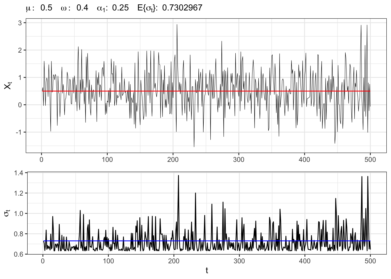
1.2 Example: ARCH(3) process
Let’s simulate an ARCH(3) process with normal residuals, namely \(X_t \sim ARCH(3)\), i.e. \[ \begin{aligned} & {} x_t = \mu + e_t \\ & e_t = \sigma_t u_t \\ & \sigma_t^{2} = \omega + \alpha_1 e_{t-1}^2 + \alpha_2 e_{t-2}^2 + \alpha_3 e_{t-3}^2 \end{aligned} \] where \(u_t \sim \mathcal{N}(0,1)\).
ARCH(3) simulation
# Random seed
set.seed(2)
# ==================== Setups =====================
# Number of simulations
t_bar <- 500
# Parameters
par <- c(mu=0.5, omega=0.4,
         alpha1=0.25, alpha2=0.05,alpha3=0.02)
# Long-term std deviation of residuals
sigma_eps <- sqrt(par[2]/(1-sum(par[3:5])))
# ================== Simulation ===================
# Initial point
Xt <- rep(par[1], 3)
# Store stochastic variance
sigma <- rep(sigma_eps, 3)
# Simulated residuals
eps <- rnorm(t_bar, 0, 1)
for(t in 4:t_bar){
  # ARCH(3) variance
  sigma[t] <- par[3]*eps[t-1]^2 + par[4]*eps[t-2]^2 + par[5]*eps[t-3]^2
  # ARCH(3) std. deviation
  sigma[t] <- sqrt(par[2] + sigma[t])
  # Simulated residuals
  eps[t] <- sigma[t]*eps[t]
  # Simulated time series
  Xt[t] <- par[1] + eps[t]
}
# ===================== Plot ======================
# ARCH(3) simulation
plot_arch <- ggplot()+
  geom_line(aes(1:t_bar, Xt), size = 0.2)+
  geom_line(aes(1:t_bar, par[1]), color = "red")+
  theme_bw()+
  labs(x = NULL, y = TeX("$X_t$"),
       subtitle = TeX(paste0("$\\mu:\\;", par[1],
                             "\\;\\; \\omega:\\;", par[2],
                             "\\;\\; \\alpha_{1}:\\;", par[3],
                             "\\;\\; \\alpha_{2}:\\;", par[4],
                             "\\;\\; \\alpha_{3}:\\;", par[5],
                             "\\;\\; E\\{\\sigma_t\\}:\\;", sigma_eps,
                             "$")))
# ARCH(3) std. deviation
plot_sigma <- ggplot()+
  geom_line(aes(1:t_bar, sigma), alpha = 1)+
  geom_line(aes(1:t_bar, sigma_eps), alpha = 1, color = "blue")+
  labs(x = "t", y = TeX("$\\sigma_{t}$"))+
  theme_bw()
gridExtra::grid.arrange(plot_arch, plot_sigma, heights = c(0.6, 0.4))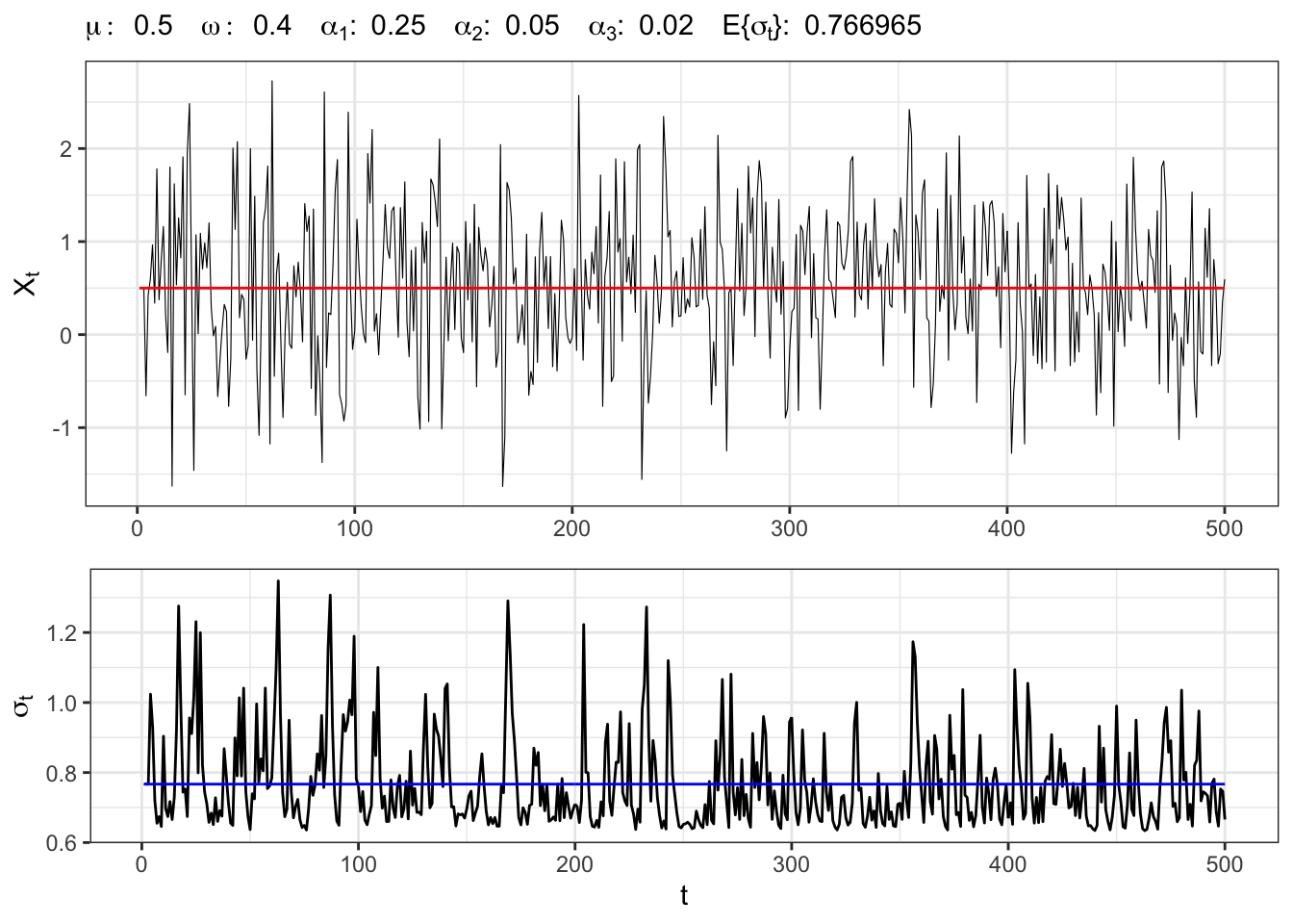
2 GARCH(p,q) process
As done with the ARCH(p), with generalized autoregressive conditional heteroskedasticity (GARCH) we model the dependency of the conditional second moment. It represents a more parsimonious way to express the conditional variance. Let’s consider a process \(X_t \sim \text{GARCH}(p,q)\), then it is defined as: \[ \begin{aligned} & {} x_t = \mu + e_t \\ & e_t = \sigma_t u_t \\ & \sigma_t^{2} = \omega + \sum_{i=1}^{p} \alpha_i e_{t-i}^2 + \sum_{j=1}^{q} \beta_j \sigma_{t-j}^2 \end{aligned} \] where \(u_t \sim \text{MDS}(0,1)\).
The unconditional and conditional mean of a process \(X_t \sim GARCH(p,q)\) are equal to: \[
\mathbb{E}\{X_t\} = \mathbb{E}\{X_t|I_{t-1}\} = \mu \text{,}
\] where \(I_{t-1}\) denotes the information available up to time \(t-1\). Instead, the long term variance of the process, i.e. the unconditional variance, is defined as for the ARCH(p) model:
\[
\mathbb{V}\{X_t\} = \mathbb{E}\{\sigma_t^2\}
\] where what changes is the unconditional expectation of the stochastic variance i.e. \[
\mathbb{E}\{\sigma_t^2\} = \frac{\omega}{1 - \sum_{i=1}^{p} \alpha_i - \sum_{j=1}^{q} \beta_j} \text{.}
\] It is clear that, in general \(\omega \neq 0\) and, to ensure that the process is stationary, the following condition on the parameters must be satisfied: \[
\sum_{i=1}^{p} \alpha_i + \sum_{j=1}^{q} \beta_j < 1 \quad \alpha_i, \beta_j > 0 \;\; \forall i, \forall j \text{.}
\]
2.1 Example: GARCH(1,1) process
Let’s simulate an GARCH(1,1) process with normal residuals, namely \(X_t \sim GARCH(1,1)\), i.e. \[ \begin{aligned} & {} x_t = \mu + e_t \\ & e_t = \sigma_t u_t \\ & \sigma_t^{2} = \omega + \alpha_1 e_{t-1}^2 + \beta_1 \sigma_{t-1}^2 \end{aligned} \] where \(u_t \sim \mathcal{N}(0,1)\).
GARCH(1,1) simulation
# Random seed
set.seed(3)
# ==================== Setups =====================
# number of simulations
t_bar <- 500
# parameters
par <- c(mu=0.5, omega=0.4, alpha1=0.25, beta1=0.25)
# long-term std deviation of residuals
sigma_eps <- sqrt(par[2]/(1 - par[3] - par[4]))
# ================== Simulation ===================
# Initial points
Xt <- rep(par[1], 1)
sigma <- rep(sigma_eps, 1)
# Simulated residuals
eps <- rnorm(t_bar, 0, 1)
for(t in 2:t_bar){
  # GARCH(1,1) variance
  sigma[t] <- par[3]*eps[t-1]^2 + par[4]*sigma[t-1]^2
  # GARCH std. deviation
  sigma[t] <- sqrt(par[2] + sigma[t])
  # Simulated residuals
  eps[t] <- sigma[t]*eps[t]
  # Simulated time series
  Xt[t] <- par[1] + eps[t]
}
# ===================== Plot ======================
# GARCH(1,1) simulation
plot_garch <- ggplot()+
  geom_line(aes(1:t_bar, Xt), size = 0.2)+
  geom_line(aes(1:t_bar, par[1]), color = "red")+
  theme_bw()+
  labs(x = NULL, y = TeX("$X_t$"),
       subtitle = TeX(paste0("$\\mu:\\;", par[1],
                             "\\;\\; \\omega:\\;", par[2],
                             "\\;\\; \\alpha_{1}:\\;", par[3],
                             "\\;\\; \\beta_{1}:\\;", par[4],
                             "\\;\\; E\\{\\sigma_t\\}:\\;", sigma_eps,
                             "$")))
# GARCH(1,1) std. deviation
plot_sigma <- ggplot()+
  geom_line(aes(1:t_bar, sigma), alpha = 1)+
  geom_line(aes(1:t_bar, sigma_eps), alpha = 1, color = "blue")+
  labs(x = "t", y = TeX("$\\sigma_{t}$"))+
  theme_bw()
gridExtra::grid.arrange(plot_garch, plot_sigma, heights = c(0.6, 0.4))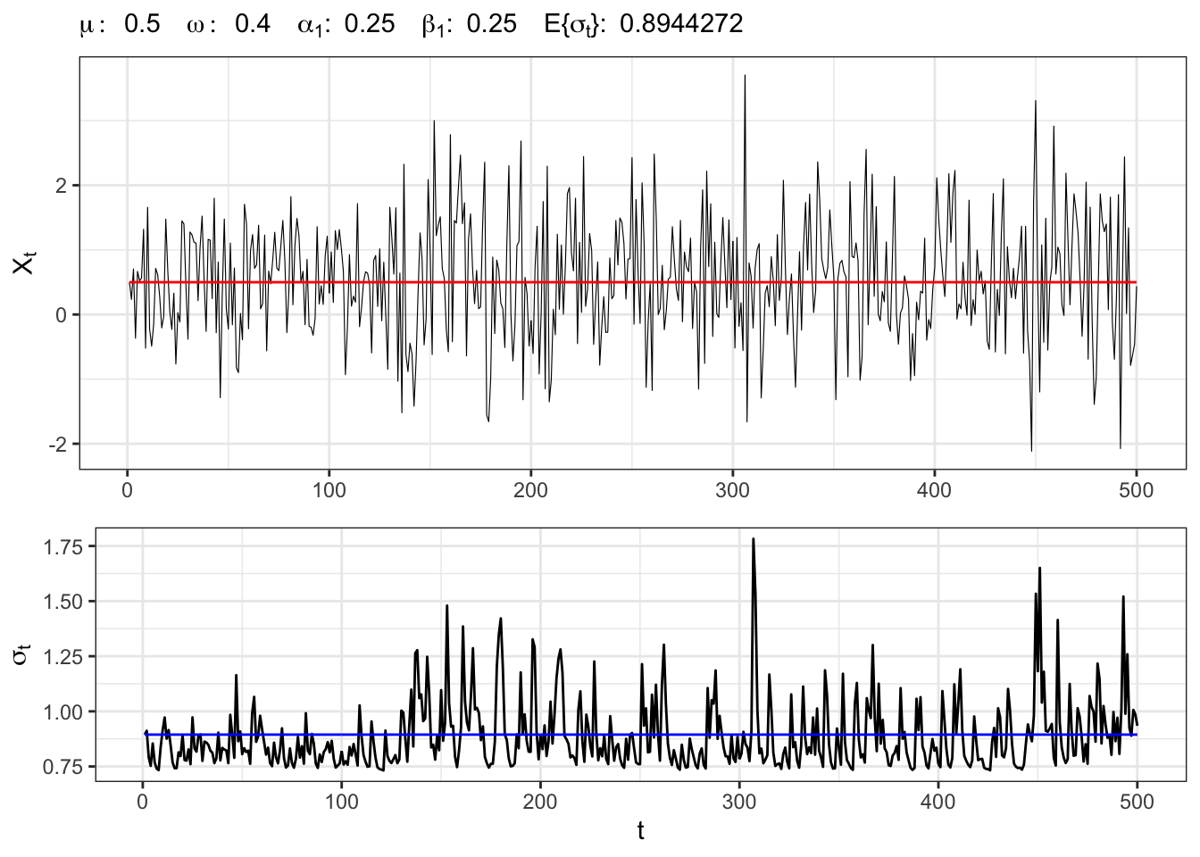
2.2 Example: GARCH(2,3) process
Let’s simulate an GARCH(2,3) process with normal residuals, namely \(X_t \sim GARCH(2,3)\), i.e. \[ \begin{aligned} & {} x_t = \mu + e_t \\ & e_t = \sigma_t u_t \\ & \sigma_t^{2} = \omega + \sum_{i=1}^{2} \alpha_i e_{t-i}^2 + \sum_{j=1}^{3} \beta_j \sigma_{t-j}^2 \end{aligned} \] where \(u_t \sim \mathcal{N}(0,1)\).
GARCH(2,3) simulation
# Random seed
set.seed(4)
# ==================== Setups =====================
# Number of simulations
t_bar <- 500
# Parameters
par <- c(mu=0.5, omega=0.4,
         alpha1=0.05, alpha1=0.03,
         beta1=0.55, beta2=0.15, beta3=0.05)
# Long-term std deviation of residuals
sigma_eps <- sqrt(par[2]/(1 - sum(par[3:7])))
# ================== Simulation ===================
# Initial points
Xt <- rep(par[1], 4)
sigma <- rep(sigma_eps, 4)
# Simulated residuals
eps <- rnorm(t_bar, 0, 1)
for(t in 4:t_bar){
  # ARCH(2) variance
  sigma2_arch <- par[3]*eps[t-1]^2 + par[4]*eps[t-2]^2
  # GARCH(3) variance
  sigma2_garch <- par[5]*sigma[t-1]^2 + par[6]*sigma[t-2]^2 + par[7]*sigma[t-3]^2
  # GARCH(2,3) std. deviation
  sigma[t] <- sqrt(par[2] + sigma2_arch + sigma2_garch)
  # Simulated residuals
  eps[t] <- sigma[t]*eps[t]
  # Simulated time series
  Xt[t] <- par[1] + eps[t]
}
# ===================== Plot ======================
# GARCH(2,3) simulation
plot_garch <- ggplot()+
  geom_line(aes(1:t_bar, Xt), size = 0.2)+
  geom_line(aes(1:t_bar, par[1]), color = "red")+
  theme_bw()+
  labs(x = NULL, y = TeX("$X_t$"),
       subtitle = TeX(paste0("$\\mu:\\;", par[1],
                             "\\;\\; \\omega:\\;", par[2],
                             "\\;\\; \\alpha_{1}:\\;", par[3],
                             "\\;\\; \\alpha_{2}:\\;", par[4],
                             "\\;\\; \\beta_{1}:\\;", par[5],
                             "\\;\\; \\beta_{2}:\\;", par[6],
                             "\\;\\; \\beta_{3}:\\;", par[7],
                             "\\;\\; E\\{\\sigma_t\\}:\\;", sigma_eps,
                             "$")))
# GARCH(2,3) std. deviation
plot_sigma <- ggplot()+
  geom_line(aes(1:t_bar, sigma), alpha = 1)+
  geom_line(aes(1:t_bar, sigma_eps), color = "blue")+
  labs(x = "t", y = TeX("$\\sigma_{t}$"))+
  theme_bw()
gridExtra::grid.arrange(plot_garch, plot_sigma, heights = c(0.6, 0.4))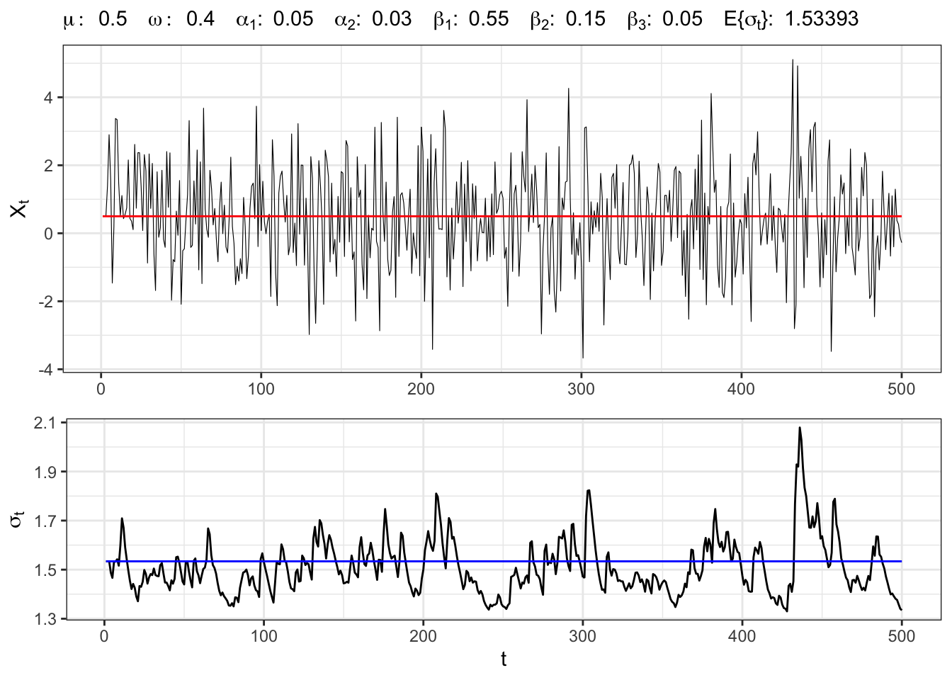
2.3 Example: GARCH(3,2) process
Let’s simulate an GARCH(3,2) process with normal residuals, namely \(X_t \sim GARCH(3,2)\), i.e. \[ \begin{aligned} & {} x_t = \mu + e_t \\ & e_t = \sigma_t u_t \\ & \sigma_t^{2} = \omega + \sum_{i=1}^{3} \alpha_i e_{t-i}^2 + \sum_{j=1}^{2} \beta_j \sigma_{t-j}^2 \end{aligned} \] where \(u_t \sim \mathcal{N}(0,1)\).
GARCH(3,2) simulation
# Random seed
set.seed(5)
# ==================== Setups =====================
# Number of simulations
t_bar <- 500
# Parameters
par <- c(mu = 0.5, omega = 0.1, alpha1 = 0.55,
         alpha2 = 0.15, alpha3 = 0.05,
         beta1 = 0.05, beta2 = 0.03)
# Long-term std deviation of residuals
sigma_eps <- sqrt(par[2]/(1 - sum(par[3:7])))
# ================== Simulation ===================
# Initial points
Xt <- rep(par[1], 4)
sigma <- rep(sigma_eps, 4)
# Simulated residuals
eps <- rnorm(t_bar, 0, 1)
for(t in 4:t_bar){
  # ARCH(3) variance
  sigma2_arch <- par[3]*eps[t-1]^2 + par[4]*eps[t-2]^2 + par[5]*eps[t-3]^2
  # GARCH(2) variance
  sigma2_garch <- par[6]*sigma[t-3]^2 + par[7]*sigma[t-2]^2
  # GARCH(3,2) std. deviation
  sigma[t] <- sqrt(par[2] + sigma2_arch + sigma2_garch)
  # Simulated residuals
  eps[t] <- sigma[t]*eps[t]
  # Simulated time series
  Xt[t] <- par[1] + eps[t]
}
# ===================== Plot ======================
# GARCH(3,2) simulation
plot_garch <- ggplot()+
  geom_line(aes(1:t_bar, Xt), size = 0.2)+
  geom_line(aes(1:t_bar, par[1]), color = "red", size = 0.2)+
  theme_bw()+
  labs(x = NULL, y = TeX("$X_t$"),
       subtitle = TeX(paste0("$\\mu:\\;", par[1],
                             "\\;\\; \\omega:\\;", par[2],
                             "\\;\\; \\alpha_{1}:\\;", par[3],
                             "\\;\\; \\alpha_{2}:\\;", par[4],
                             "\\;\\; \\alpha_{3}:\\;", par[5],
                             "\\;\\; \\beta_{1}:\\;", par[6],
                             "\\;\\; \\beta_{2}:\\;", par[7],
                             "\\;\\; E\\{\\sigma_t\\}:\\;", sigma_eps,
                             "$")))
# GARCH(3,2) std. deviation
plot_sigma <- ggplot()+
  geom_line(aes(1:t_bar, sigma), alpha = 1)+
  geom_line(aes(1:t_bar, sigma_eps), color = "blue")+
  labs(x = "t", y = TeX("$\\sigma_{t}$"))+
  theme_bw()
gridExtra::grid.arrange(plot_garch, plot_sigma, heights = c(0.6, 0.4))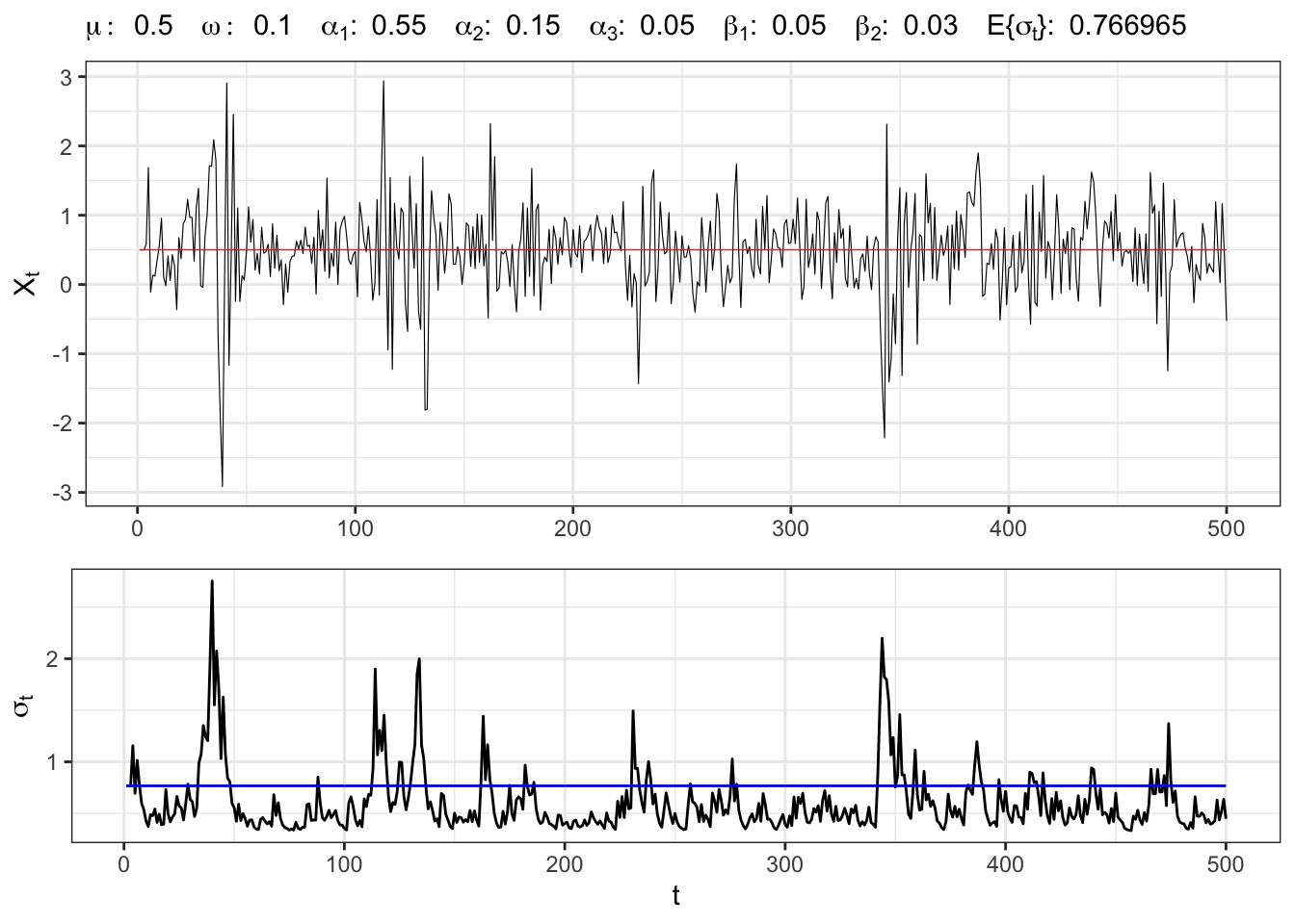
3 IGARCH
Integrated Generalized Autoregressive Conditional heteroskedasticity (IGARCH(p,q)) is a restricted version of the GARCH model, where the persistent parameters sum up to one, and imports a unit root in the GARCH process. The condition for this is
\[ \sum_{i=1}^{p} \alpha_i + \sum_{j=1}^{q} \beta_j = 1 \]
3.1 Example: IGARCH(1,1)
IGARCH(1,1) simulation
# Random seed
set.seed(6)
# ==================== Setups =====================
# number of simulations
t_bar <- 500
# parameters
par <- c(mu=0.5, omega=0.4, alpha1=0.35, beta1=0.45)
# long-term std deviation of residuals
sigma_eps <- sqrt(par[2]/(1 - par[3] - par[4]))
# ================== Simulation ===================
# Initial points
Xt <- rep(par[1], 1)
sigma <- rep(sigma_eps, 1)
# Simulated residuals
eps <- rnorm(t_bar, 0, 1)
for(t in 2:t_bar){
  # iGARCH(1,1) variance
  sigma[t] <- par[3]*eps[t-1]^2 + par[4]*sigma[t-1]^2
  # iGARCH std. deviation
  sigma[t] <- sqrt(par[2] + sigma[t])
  # Simulated residuals
  eps[t] <- sigma[t]*eps[t]
  # Simulated time series
  Xt[t] <- par[1] + eps[t]
}
# ===================== Plot ======================
# iGARCH(1,1) simulation
plot_garch <- ggplot()+
  geom_line(aes(1:t_bar, Xt), size = 0.2)+
  geom_line(aes(1:t_bar, par[1]), color = "red", size = 0.2)+
  theme_bw()+
  labs(x = NULL, y = TeX("$X_t$"),
       subtitle = TeX(paste0("$\\mu:\\;", par[1],
                             "\\;\\; \\omega:\\;", par[2],
                             "\\;\\; \\alpha_{1}:\\;", par[3],
                             "\\;\\; \\beta_{1}:\\;", par[4],
                             "\\;\\; E\\{\\sigma_t\\}:\\;", sigma_eps,
                             "$")))
# iGARCH(1,1) std. deviation
plot_sigma <- ggplot()+
  geom_line(aes(1:t_bar, sigma), alpha = 1)+
  geom_line(aes(1:t_bar, sigma_eps), alpha = 1, color = "blue")+
  labs(x = "t", y = TeX("$\\sigma_{t}$"))+
  theme_bw()
gridExtra::grid.arrange(plot_garch, plot_sigma, heights = c(0.6, 0.4))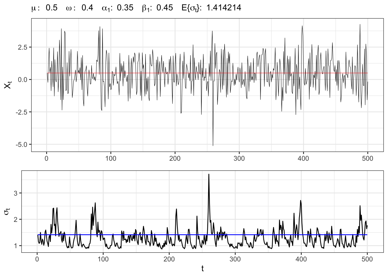
4 GARCH-M
The GARCH in-mean (GARCH-M) model adds a stochastic term into the mean equation, i.e.
\[ \begin{aligned} & {} x_t = \mu + \sigma_t \lambda + e_t \\ & e_t = \sigma_t u_t \\ & \sigma_t^{2} = \omega + \sum_{i=1}^{p} \alpha_i e_{t-i}^2 + \sum_{j=1}^{q} \beta_j \sigma_{t-j}^2 \end{aligned} \] The effect of the parameter \(\lambda\) is a shift of the mean of the process. The unconditional mean became \[ \mathbb{E}\{X_t\} = \mu + \mathbb{E}\{\sigma_t\} \lambda \]
4.1 Example: GARCH-M(1,1)
GARCH-M(1,1) simulation
set.seed(7)
# ==================== Setups =====================
# number of simulations
t_bar <- 500
# parameters
par <- c(mu=0.5, omega=0.4,
         alpha1=0.15, beta1=0.35, lambda = 1.5)
# long-term std deviation of residuals
sigma_eps <- sqrt(par[2]/(1 - par[3] - par[4]))
# ================== Simulation ===================
# Initial points
Xt <- rep(par[1], 1)
sigma <- rep(sigma_eps, 1)
# Simulated residuals
eps <- rnorm(t_bar, 0, 1)
eps[1:2] <- eps[1:2]*sigma_eps
for(t in 2:t_bar){
  # GARCH(1,1) variance
  sigma[t] <- par[3]*eps[t-1]^2 + par[4]*sigma[t-1]^2
  # GARCH std. deviation
  sigma[t] <- sqrt(par[2] + sigma[t])
  # Simulated residuals
  eps[t] <- sigma[t]*eps[t]
  # Simulated time series
  Xt[t] <- par[1] + sigma[t]*par[5] + eps[t]
}
# ===================== Plot ======================
# GARCH-M(1,1) simulation
plot_garch <- ggplot()+
  geom_line(aes(1:t_bar, Xt), size = 0.2)+
  geom_line(aes(1:t_bar, par[1] + sigma_eps*par[5]), color = "red", size = 0.2)+
  theme_bw()+
  labs(x = NULL, y = TeX("$X_t$"),
       subtitle = TeX(paste0("$\\mu:\\;", par[1],
                             "\\;\\; \\omega:\\;", par[2],
                             "\\;\\; \\alpha_{1}:\\;", par[3],
                             "\\;\\; \\beta_{1}:\\;", par[4],
                             "\\;\\; \\lambda:\\;", par[5],
                             "\\;\\; E\\{\\X_t\\}:\\;", par[1] + sigma_eps*par[5],
                             "\\;\\; E\\{\\sigma_t\\}:\\;", sigma_eps,
                             "$")))
# GARCH-M(1,1) std. deviation
plot_sigma <- ggplot()+
  geom_line(aes(1:t_bar, sigma), alpha = 1)+
  geom_line(aes(1:t_bar, sigma_eps), alpha = 1, color = "blue")+
  labs(x = "t", y = TeX("$\\sigma_{t}$"))+
  theme_bw()
gridExtra::grid.arrange(plot_garch, plot_sigma, heights = c(0.6, 0.4))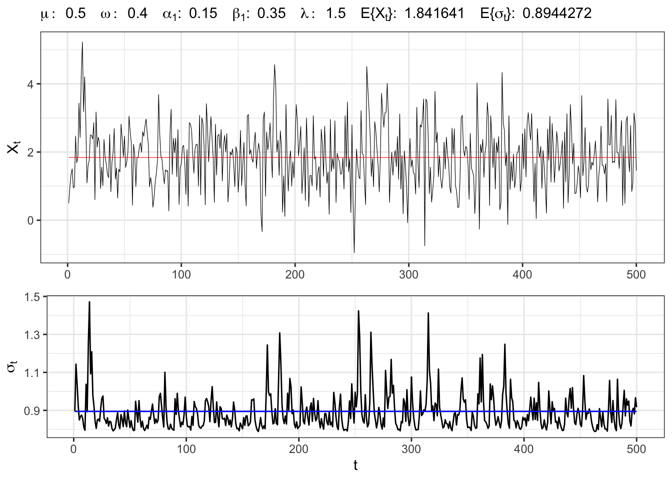
Citation
@online{sartini2024,
  author = {Sartini, Beniamino},
  title = {ARCH-GARCH Process},
  date = {2024-05-01},
  url = {https://greenfin.it/statistics/arch-garch-process.html},
  langid = {en}
}