Hourly energy demand generation and weather

1 Description of the data
The dataset contains 4 years of electrical consumption, generation, pricing, and weather data for Spain. Consumption and generation data was retrieved from ENTSOE a public portal for Transmission Service Operator (TSO) data. Settlement prices were obtained from the Spanish TSO Red Electric España. Weather data was purchased as part of a personal project from the Open Weather API for the 5 largest cities in Spain. The original datasets can be downloaded from Kaggle. However, the dataset to be used for the project has been already pre-processed. The code used for preprocessing is in this github repository, while the dataset to be used can be downloaded here.
- date: datetime index localized to CET.
- date_day: date without hour.
- city: reference city. (
Valencia.Madrid,Bilbao,Barcelona,Seville) - Year: number for the year.
- Month: number for the month.
- Day: number for the day in a month.
- Hour: reference hour of the day.
Energy variables
- fossil: energy produced with fossil sources: i.e. coal/lignite, natural gas, oil (MW).
- nuclear: energy produced with nuclear sources (MW).
- energy_other: other generation (MW).
- solar: solar generation (MW).
- biomass: biomass generation (MW).
- river: hydroeletric generation (MW).
- wind: wind generation (MW).
- energy_other_renewable: other renewable generation (MW).
- energy_waste: wasted generation (MW).
- pred_solar: forecasted solar generation (MW).
- pred_demand: forecasted electrical demand by TSO (MW).
- pred_price: forecasted day ahead electrical price by TSO (Eur/MWh).
- price: actual electrical price (Eur/MWh).
- demand: actual electrical demand (Eur/MWh).
- prod_tot: total electrical production (MW).
- prod_renewable: total renewable electrical production (MW).
Weather variables
- temp: mean temperature.
- temp_min: minimum temperature (degrees).
- temp_max: maximum temperature (degrees).
- pressure: pressure in (hPas).
- humidity: humidity in percentage.
- wind_speed: wind speed (m/s).
- wind_deg: wind direction.
- rain_1h: rain in last hour (mm).
- rain_3h: rain in last 3 hours (mm).
- snow_3h: show last 3 hours (mm).
- clouds_all: cloud cover in percentage.
Code
dir_ <- "../.."
filepath <- file.path(dir_, "databases/data/global/l0/greenfin-project/summerschool2024/data.csv")
#| code-summary: Load data
data <- readr::read_csv(filepath, show_col_types = FALSE, progress = FALSE)
head(data) %>%
  knitr::kable(booktabs = TRUE ,escape = FALSE, align = 'c')%>%
kableExtra::row_spec(0, color = "white", background = "green") | date | date_day | Year | Month | Day | Hour | Season | fossil | nuclear | energy_other | solar | biomass | river | energy_other_renewable | energy_waste | wind | pred_solar | pred_demand | pred_price | demand | price | prod | prod_renewable | temp | temp_min | temp_max | pressure | humidity | wind_speed | wind_deg | rain_1h | rain_3h | snow_3h | clouds_all |
|---|---|---|---|---|---|---|---|---|---|---|---|---|---|---|---|---|---|---|---|---|---|---|---|---|---|---|---|---|---|---|---|---|---|
| 2014-12-31 23:00:00 | 2014-12-31 | 2014 | 12 | 31 | 23 | Winter | 10156 | 7096 | 43 | 49 | 447 | 3813 | 73 | 196 | 6378 | 17 | 26118 | 50.10 | 25385 | 65.41 | 27939 | 10687 | -0.6585375 | -5.825 | 8.475 | 1016.4 | 82.4 | 2.0 | 135.2 | 0 | 0 | 0 | 0 |
| 2015-01-01 00:00:00 | 2015-01-01 | 2015 | 1 | 1 | 0 | Winter | 10437 | 7096 | 43 | 50 | 449 | 3587 | 71 | 195 | 5890 | 16 | 24934 | 48.10 | 24382 | 64.92 | 27509 | 9976 | -0.6373000 | -5.825 | 8.475 | 1016.2 | 82.4 | 2.0 | 135.8 | 0 | 0 | 0 | 0 |
| 2015-01-01 01:00:00 | 2015-01-01 | 2015 | 1 | 1 | 1 | Winter | 9918 | 7099 | 43 | 50 | 448 | 3508 | 73 | 196 | 5461 | 8 | 23515 | 47.33 | 22734 | 64.48 | 26484 | 9467 | -1.0508625 | -6.964 | 8.136 | 1016.8 | 82.0 | 2.4 | 119.0 | 0 | 0 | 0 | 0 |
| 2015-01-01 02:00:00 | 2015-01-01 | 2015 | 1 | 1 | 2 | Winter | 8859 | 7098 | 43 | 50 | 438 | 3231 | 75 | 191 | 5238 | 2 | 22642 | 42.27 | 21286 | 59.32 | 24914 | 8957 | -1.0605312 | -6.964 | 8.136 | 1016.6 | 82.0 | 2.4 | 119.2 | 0 | 0 | 0 | 0 |
| 2015-01-01 03:00:00 | 2015-01-01 | 2015 | 1 | 1 | 3 | Winter | 8313 | 7097 | 43 | 42 | 428 | 3499 | 74 | 189 | 4935 | 9 | 21785 | 38.41 | 20264 | 56.04 | 24314 | 8904 | -1.0041000 | -6.964 | 8.136 | 1016.6 | 82.0 | 2.4 | 118.4 | 0 | 0 | 0 | 0 |
| 2015-01-01 04:00:00 | 2015-01-01 | 2015 | 1 | 1 | 4 | Winter | 7962 | 7098 | 43 | 34 | 410 | 3804 | 74 | 188 | 4618 | 4 | 21441 | 35.72 | 19905 | 53.63 | 23926 | 8866 | -1.1260000 | -7.708 | 7.317 | 1017.4 | 82.6 | 2.4 | 174.8 | 0 | 0 | 0 | 0 |
2 Project
2.1 Problem A. Explorative analysis
Consider the data of the energy market in Spain and let’s examine the composition of the energy mix. At your disposal you have 5 sources that generate energy, i.e. 4 renewable (columns biomass, solar, river, wind) and 2 non-renewable (columns nuclear, fossil). The column demand denotes the amount of demanded electricity in MW, instead the column price denotes the actual price in \(MW/h\). For simplicity, let’s denote with \(E^{\boldsymbol{\ast}}_{t}\) the energy of the \(\boldsymbol{\ast}\)-th source, i.e. \[
E^{\boldsymbol{\ast}}_{t} =
\begin{cases}
E^{b}_{t} \quad \boldsymbol{\ast} \to b = \text{biomass} \\
E^{s}_{t} \quad \boldsymbol{\ast} \to s = \text{solar} \\
E^{h}_{t} \quad \boldsymbol{\ast} \to h = \text{hydroelettric} \\
E^{w}_{t} \quad \boldsymbol{\ast} \to w = \text{wind} \\
E^{n}_{t} \quad \boldsymbol{\ast} \to n = \text{nuclear} \\
E^{f}_{t} \quad \boldsymbol{\ast} \to f = \text{fossil} \\
\end{cases}
\] and the total energy demanded at time \(t\) as \(D_t\).
2.1.1 Task A.1
Compute the average between the energy produced from each source and the total demand, i.e.
\[
R^{{\boldsymbol{\ast}}} = \frac{1}{n} \sum_{t = 1}^{n} \frac{E^{\boldsymbol{\ast}}_{t}}{D_{t}}
\tag{1}\]
and normalize them, i.e. \(R^{\boldsymbol{\ast}}/\sum R^{\boldsymbol{\ast}}\). Rank the 5 sources of energy by the percentage of demand satisfied in decreasing order and plot the values obtained with histograms.
Code
var_levels <- c("biomass", "solar", "hydroelettric", "wind", "nuclear", "fossil")
var_labels <- c("Biomass", "Solar", "Hydroelettric", "Wind", "Nuclear", "Fossil")
# Compute the percentage ratio
df_A1 <- data %>%
  dplyr::summarise(biomass = mean(biomass/demand),
                   solar = mean(solar/demand),
                   hydroelettric = mean(river/demand),
                   wind = mean(wind/demand),
                   nuclear = mean(nuclear/demand),
                   fossil = mean(fossil/demand))%>%
  tidyr::gather(key = "source", value = "perc")
# Categorical variable (plots purposes)
df_A1$id <- factor(df_A1$source, levels = var_levels, labels = var_labels)
# Normalize the percentages
df_A1$perc <- df_A1$perc/sum(df_A1$perc)

# Rank the sources
vec_max <- df_A1$perc
names(vec_max) <- var_labels
vec_max_sort <- vec_max[order(vec_max, decreasing = TRUE)]Code
df_A1 %>%
  ggplot()+
  geom_bar(aes(id, perc, fill = source), color = "black", stat = "identity")+
  theme_bw()+
  custom_theme+
  theme(legend.position = "none")+
  scale_fill_manual(values = c(fossil = "#65880f", nuclear = "#0477BF", biomass = "brown",
                               solar = "darkorange", hydroelettric = "blue", wind = "gray"))+
  scale_y_continuous(breaks = seq(0, 1, 0.05),
                     labels = paste0(seq(0, 1, 0.05)*100, " %"))+
  labs(fill = NULL, x = NULL, y = NULL)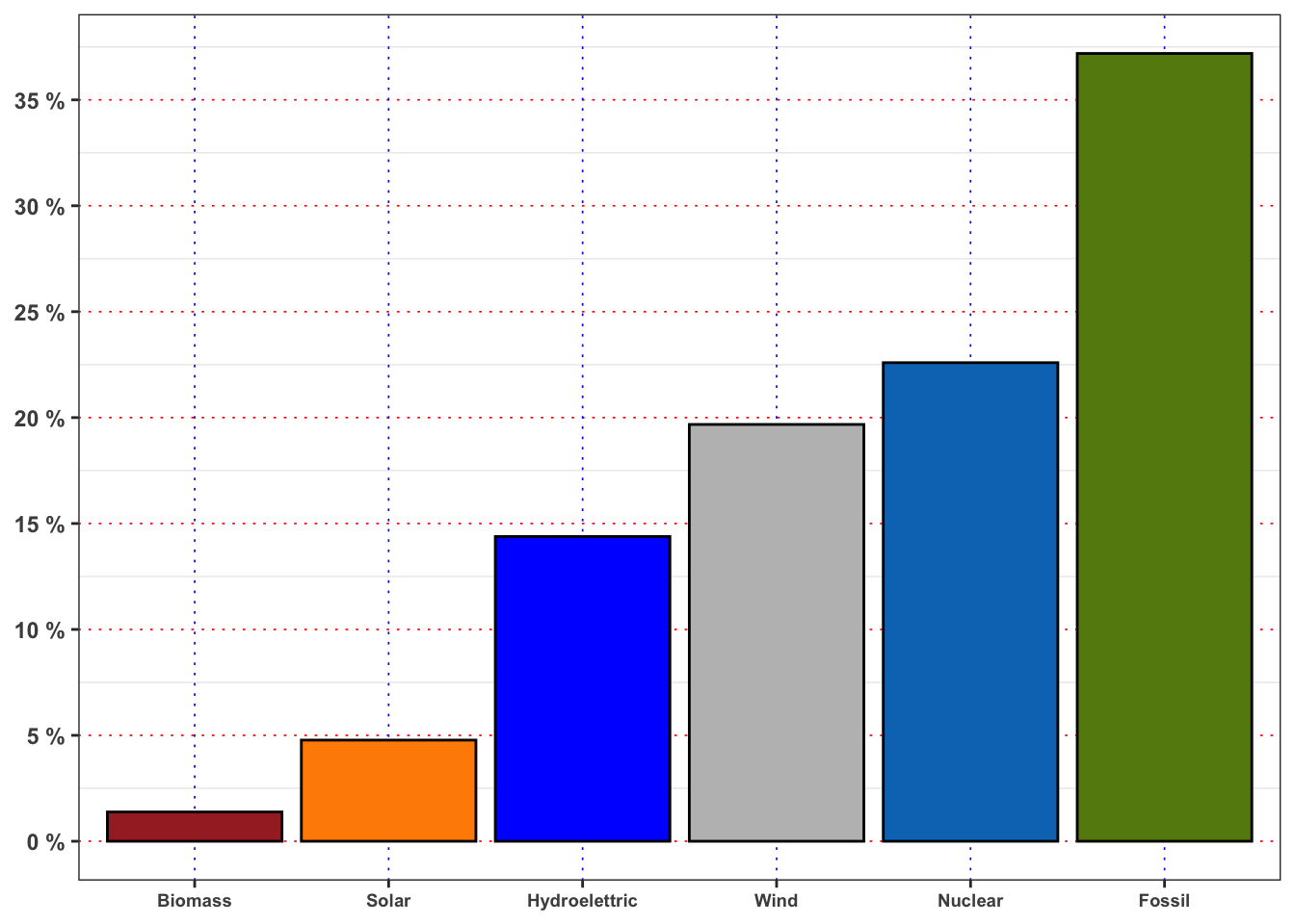
The 1° source with respect to production/demand is Fossil (37.19%). The 2° source with respect to production/demand is Nuclear (22.59%). The 3° source with respect to production/demand is Wind (19.68%). The 4° source with respect to production/demand is Hydroelettric (14.39%). The 5° source with respect to production/demand is Solar (4.78%). The 6° source with respect to production/demand is Biomass (1.38%).
2.1.2 Task A.2
Aggregate the sources of energy in two groups:
- Renewable: is given by the sum of
solar,river,windandbiomass. - Non-renewable: is given by the sum of
nuclearandfossil.
Then, compute the percentage of energy demand satisfied by each group. What is the percentage of energy satisfied by renewable sources? And by the fossil ones?
Repeat the computations, but filtering the data firstly only for year 2015 and then only for 2018. Are the percentage obtained different? Describe the result and explain if the transition to renewable energy is supported by data (to be supported the percentage of renewable energy should increase while percentage of fossil fuels should decrease.)
The percentage of demand satisfied by renewable sources is 40.22 %. Instead, the percentage of demand satisfied by fossil and nuclear sources is 59.78 %. The ratio of the fossil plus nuclear is 48.65 % bigger with respect to renewable sources.
Code
# Percentage of demand by source in 2015
df_A2_2015 <- data %>%
  filter(Year == 2015) %>%
  summarise(biomass = mean(biomass/demand, na.rm = TRUE),
            solar = mean(solar/demand, na.rm = TRUE),
            river = mean(river/demand, na.rm = TRUE),
            wind = mean(wind/demand, na.rm = TRUE),
            nuclear = mean(nuclear/demand, na.rm = TRUE),
            fossil = mean(fossil/demand, na.rm = TRUE))%>%
  gather(key = "source", value = "perc")
# Normalize
df_A2_2015$perc <- df_A2_2015$perc/sum(df_A2_2015$perc)
# Categorical variable (plots purposes)
df_A2_2015$id <- factor(df_A2_2015$source, levels = var_levels, labels = var_labels)

# Percentage of demand by source in 2018
df_A2_2018 <- data %>%
  filter(Year == 2018) %>%
  summarise(biomass = mean(biomass/demand, na.rm = TRUE),
            solar = mean(solar/demand, na.rm = TRUE),
            river = mean(river/demand, na.rm = TRUE),
            wind = mean(wind/demand, na.rm = TRUE),
            nuclear = mean(nuclear/demand, na.rm = TRUE),
            fossil = mean(fossil/demand, na.rm = TRUE))%>%
  gather(key = "source", value = "perc")
# Normalize
df_A2_2018$perc <- df_A2_2018$perc/sum(df_A2_2018$perc)
# Categorical variable (plots purposes)
df_A2_2018$id <- factor(df_A2_2018$source, levels = var_levels, labels = var_labels)
Code
response <- paste0(
  "In 2015 the percentage of demand satisfied by renewable sources was ",
  round(sum(df_A2_2015$perc[1:4])*100, 3), " %, while in 2019 was ",
  round(sum(df_A2_2018$perc[1:4])*100, 3), " %. ",
  "Hence, the dominance of renewable sources in this period increased by ",
  round((sum(df_A2_2018$perc[1:4])/sum(df_A2_2015$perc[1:4])-1)*100, 3), " %.",
  " Instead, in 2015 the percentage of demand satisfied by fossil and nuclear sources was ",
  round(sum(df_A2_2015$perc[5:6])*100, 3), " %, while in 2019 was ",
  round(sum(df_A2_2018$perc[5:6])*100, 3), " %. ",
  "Hence, the dominance of fossil sources in this period decreased by ",
  round((sum(df_A2_2018$perc[5:6])/sum(df_A2_2015$perc[5:6])-1)*100, 3),
  " %. and the transition seems to be supported by data."
)
In 2015 the percentage of demand satisfied by renewable sources was 39.335 %, while in 2019 was 42.132 %. Hence, the dominance of renewable sources in this period increased by 7.111 %. Instead, in 2015 the percentage of demand satisfied by fossil and nuclear sources was 60.665 %, while in 2019 was 57.868 %. Hence, the dominance of fossil sources in this period decreased by -4.611 %. and the transition seems to be supported by data.
2.1.3 Task A.3
For each month, compute the mean percentage of demand of energy satisfied by the fossil sources. In order to compute \(R^{{\boldsymbol{\ast}}}_m\) for the \(m\)-month, let’s denote with \(n_m\) the number of day in that month, then: \[ R^{{\boldsymbol{\ast}}}_m = \frac{1}{n_m} \sum_{t = 1}^{n_m} \frac{E^{\boldsymbol{\ast}}_{t}}{D_{t}} = \frac{1}{n_m} \sum_{t = 1}^{n_m} R^{{\boldsymbol{\ast}}}_t \tag{2}\]
Compute also the maximum, minimum, median and standard deviation of \(R^{{\boldsymbol{\ast}}}_t\) for each month. Repeat the computation for the others 4 sources of energy, i.e. nuclear, solar, river and wind. Which are the source with the lowest and the highest standard deviation in December? And in June? Comment the results obtained (max 200 words).
| Month | min | mean | meadian | max | sd |
|---|---|---|---|---|---|
| Jan | 10.607 % | 36.87 % | 38.61 % | 66.58 % | 10.082 % |
| Feb | 9.125 % | 32.48 % | 32.21 % | 67.95 % | 11.214 % |
| Mar | 13.351 % | 29.39 % | 26.56 % | 69.18 % | 10.438 % |
| Apr | 12.396 % | 31.03 % | 28.80 % | 70.62 % | 11.246 % |
| May | 9.976 % | 33.35 % | 33.01 % | 76.60 % | 10.764 % |
| Jun | 12.730 % | 36.97 % | 37.35 % | 75.26 % | 11.359 % |
| Jul | 14.677 % | 39.85 % | 40.64 % | 63.78 % | 9.407 % |
| Aug | 13.075 % | 38.00 % | 38.82 % | 60.91 % | 8.791 % |
| Sep | 12.927 % | 39.40 % | 40.53 % | 68.04 % | 9.156 % |
| Oct | 12.531 % | 41.37 % | 41.69 % | 72.10 % | 10.998 % |
| Nov | 12.924 % | 44.10 % | 45.71 % | 78.15 % | 12.626 % |
| Dec | 13.891 % | 38.77 % | 39.69 % | 67.38 % | 11.030 % |
| Month | min | mean | meadian | max | sd |
|---|---|---|---|---|---|
| Jan | 12.271 % | 22.74 % | 21.86 % | 39.22 % | 4.498 % |
| Feb | 11.660 % | 22.56 % | 21.77 % | 38.42 % | 4.655 % |
| Mar | 13.040 % | 23.46 % | 22.74 % | 36.57 % | 4.504 % |
| Apr | 12.624 % | 23.13 % | 22.65 % | 37.64 % | 4.906 % |
| May | 4.999 % | 20.40 % | 19.98 % | 37.59 % | 3.990 % |
| Jun | 12.569 % | 21.17 % | 20.67 % | 37.76 % | 4.381 % |
| Jul | 12.390 % | 21.65 % | 21.09 % | 34.93 % | 3.956 % |
| Aug | 12.780 % | 23.61 % | 23.08 % | 34.00 % | 4.113 % |
| Sep | 13.929 % | 23.65 % | 22.98 % | 35.29 % | 4.348 % |
| Oct | 14.127 % | 23.09 % | 22.54 % | 35.85 % | 4.503 % |
| Nov | 0.000 % | 19.82 % | 19.25 % | 33.38 % | 4.343 % |
| Dec | 13.425 % | 23.08 % | 22.31 % | 39.37 % | 5.219 % |
| Month | min | mean | meadian | max | sd |
|---|---|---|---|---|---|
| Jan | 1.1883 % | 21.80 % | 20.39 % | 62.26 % | 11.609 % |
| Feb | 1.5627 % | 22.85 % | 21.24 % | 61.05 % | 13.511 % |
| Mar | 1.5243 % | 24.03 % | 23.67 % | 64.02 % | 12.726 % |
| Apr | 1.8202 % | 20.14 % | 18.09 % | 64.49 % | 11.326 % |
| May | 1.1022 % | 19.88 % | 17.45 % | 57.96 % | 11.555 % |
| Jun | 1.0185 % | 18.12 % | 15.68 % | 65.36 % | 10.978 % |
| Jul | 0.6918 % | 15.96 % | 14.27 % | 59.08 % | 9.259 % |
| Aug | 0.7066 % | 16.75 % | 15.52 % | 57.37 % | 9.134 % |
| Sep | 0.9261 % | 16.05 % | 13.60 % | 56.38 % | 10.383 % |
| Oct | 0.7795 % | 19.22 % | 16.83 % | 62.57 % | 12.014 % |
| Nov | 0.0000 % | 18.93 % | 16.16 % | 69.16 % | 12.136 % |
| Dec | 1.6081 % | 20.17 % | 18.12 % | 67.28 % | 12.108 % |
| Month | min | mean | meadian | max | sd |
|---|---|---|---|---|---|
| Jan | 2.983 % | 15.06 % | 13.798 % | 41.58 % | 6.731 % |
| Feb | 3.003 % | 17.33 % | 16.062 % | 42.13 % | 7.674 % |
| Mar | 2.540 % | 18.69 % | 18.987 % | 45.22 % | 7.715 % |
| Apr | 2.928 % | 18.84 % | 16.437 % | 49.09 % | 9.524 % |
| May | 2.858 % | 16.92 % | 15.327 % | 50.66 % | 8.092 % |
| Jun | 2.796 % | 13.81 % | 13.050 % | 38.07 % | 5.839 % |
| Jul | 2.261 % | 11.50 % | 10.293 % | 40.04 % | 5.887 % |
| Aug | 3.040 % | 10.94 % | 9.488 % | 43.30 % | 6.013 % |
| Sep | 2.635 % | 11.05 % | 9.611 % | 36.30 % | 5.534 % |
| Oct | 2.271 % | 11.61 % | 10.175 % | 44.41 % | 6.266 % |
| Nov | 0.000 % | 12.28 % | 11.021 % | 43.45 % | 6.441 % |
| Dec | 3.519 % | 13.11 % | 11.911 % | 46.06 % | 6.121 % |
| Month | min | mean | meadian | max | sd |
|---|---|---|---|---|---|
| Jan | 0.024068 % | 3.523 % | 0.7840 % | 25.38 % | 4.830 % |
| Feb | 0.006935 % | 3.966 % | 1.3321 % | 22.70 % | 5.080 % |
| Mar | 0.018776 % | 4.517 % | 2.0257 % | 21.22 % | 5.345 % |
| Apr | 0.009580 % | 4.986 % | 2.3468 % | 21.88 % | 5.572 % |
| May | 0.008510 % | 5.942 % | 3.0158 % | 22.48 % | 5.939 % |
| Jun | 0.011501 % | 6.248 % | 3.2706 % | 22.03 % | 5.761 % |
| Jul | 0.008478 % | 6.221 % | 2.9958 % | 23.40 % | 5.726 % |
| Aug | 0.009806 % | 5.774 % | 2.6587 % | 21.32 % | 5.825 % |
| Sep | 0.017305 % | 5.333 % | 2.2467 % | 23.02 % | 5.875 % |
| Oct | 0.007038 % | 3.767 % | 1.0721 % | 21.75 % | 4.974 % |
| Nov | 0.000000 % | 3.355 % | 0.6537 % | 18.63 % | 4.619 % |
| Dec | 0.008983 % | 3.063 % | 0.4059 % | 19.26 % | 4.386 % |
Code
create_monthly_kable(data, target = "biomass")
## $data
## # A tibble: 12 × 6
##    Month     min   mean meadian    max      sd
##    <ord>   <dbl>  <dbl>   <dbl>  <dbl>   <dbl>
##  1 Jan   0.00732 0.0140  0.0138 0.0263 0.00350
##  2 Feb   0.00623 0.0139  0.0138 0.0274 0.00307
##  3 Mar   0.00476 0.0133  0.0131 0.0268 0.00406
##  4 Apr   0.00608 0.0119  0.0115 0.0282 0.00349
##  5 May   0       0.0139  0.0131 0.0272 0.00370
##  6 Jun   0.00675 0.0134  0.0128 0.0261 0.00348
##  7 Jul   0.00694 0.0136  0.0131 0.0272 0.00327
##  8 Aug   0.00527 0.0145  0.0137 0.0286 0.00378
##  9 Sep   0.00599 0.0142  0.0135 0.0281 0.00383
## 10 Oct   0.00543 0.0140  0.0131 0.0289 0.00403
## 11 Nov   0       0.0137  0.0130 0.0283 0.00372
## 12 Dec   0.00580 0.0134  0.0128 0.0280 0.00366
##
## $kab
## <table>
##  <thead>
##   <tr>
##    <th style="text-align:left;"> Month </th>
##    <th style="text-align:left;"> min </th>
##    <th style="text-align:left;"> mean </th>
##    <th style="text-align:left;"> meadian </th>
##    <th style="text-align:left;"> max </th>
##    <th style="text-align:left;"> sd </th>
##   </tr>
##  </thead>
## <tbody>
##   <tr>
##    <td style="text-align:left;"> Jan </td>
##    <td style="text-align:left;"> 0.7321 % </td>
##    <td style="text-align:left;"> 1.404 % </td>
##    <td style="text-align:left;"> 1.383 % </td>
##    <td style="text-align:left;"> 2.630 % </td>
##    <td style="text-align:left;"> 0.3501 % </td>
##   </tr>
##   <tr>
##    <td style="text-align:left;"> Feb </td>
##    <td style="text-align:left;"> 0.6226 % </td>
##    <td style="text-align:left;"> 1.394 % </td>
##    <td style="text-align:left;"> 1.380 % </td>
##    <td style="text-align:left;"> 2.741 % </td>
##    <td style="text-align:left;"> 0.3070 % </td>
##   </tr>
##   <tr>
##    <td style="text-align:left;"> Mar </td>
##    <td style="text-align:left;"> 0.4760 % </td>
##    <td style="text-align:left;"> 1.334 % </td>
##    <td style="text-align:left;"> 1.306 % </td>
##    <td style="text-align:left;"> 2.680 % </td>
##    <td style="text-align:left;"> 0.4059 % </td>
##   </tr>
##   <tr>
##    <td style="text-align:left;"> Apr </td>
##    <td style="text-align:left;"> 0.6078 % </td>
##    <td style="text-align:left;"> 1.191 % </td>
##    <td style="text-align:left;"> 1.147 % </td>
##    <td style="text-align:left;"> 2.819 % </td>
##    <td style="text-align:left;"> 0.3495 % </td>
##   </tr>
##   <tr>
##    <td style="text-align:left;"> May </td>
##    <td style="text-align:left;"> 0.0000 % </td>
##    <td style="text-align:left;"> 1.394 % </td>
##    <td style="text-align:left;"> 1.308 % </td>
##    <td style="text-align:left;"> 2.718 % </td>
##    <td style="text-align:left;"> 0.3703 % </td>
##   </tr>
##   <tr>
##    <td style="text-align:left;"> Jun </td>
##    <td style="text-align:left;"> 0.6752 % </td>
##    <td style="text-align:left;"> 1.344 % </td>
##    <td style="text-align:left;"> 1.277 % </td>
##    <td style="text-align:left;"> 2.614 % </td>
##    <td style="text-align:left;"> 0.3477 % </td>
##   </tr>
##   <tr>
##    <td style="text-align:left;"> Jul </td>
##    <td style="text-align:left;"> 0.6938 % </td>
##    <td style="text-align:left;"> 1.365 % </td>
##    <td style="text-align:left;"> 1.305 % </td>
##    <td style="text-align:left;"> 2.719 % </td>
##    <td style="text-align:left;"> 0.3265 % </td>
##   </tr>
##   <tr>
##    <td style="text-align:left;"> Aug </td>
##    <td style="text-align:left;"> 0.5274 % </td>
##    <td style="text-align:left;"> 1.447 % </td>
##    <td style="text-align:left;"> 1.373 % </td>
##    <td style="text-align:left;"> 2.859 % </td>
##    <td style="text-align:left;"> 0.3776 % </td>
##   </tr>
##   <tr>
##    <td style="text-align:left;"> Sep </td>
##    <td style="text-align:left;"> 0.5987 % </td>
##    <td style="text-align:left;"> 1.424 % </td>
##    <td style="text-align:left;"> 1.348 % </td>
##    <td style="text-align:left;"> 2.809 % </td>
##    <td style="text-align:left;"> 0.3834 % </td>
##   </tr>
##   <tr>
##    <td style="text-align:left;"> Oct </td>
##    <td style="text-align:left;"> 0.5433 % </td>
##    <td style="text-align:left;"> 1.404 % </td>
##    <td style="text-align:left;"> 1.314 % </td>
##    <td style="text-align:left;"> 2.890 % </td>
##    <td style="text-align:left;"> 0.4034 % </td>
##   </tr>
##   <tr>
##    <td style="text-align:left;"> Nov </td>
##    <td style="text-align:left;"> 0.0000 % </td>
##    <td style="text-align:left;"> 1.372 % </td>
##    <td style="text-align:left;"> 1.298 % </td>
##    <td style="text-align:left;"> 2.830 % </td>
##    <td style="text-align:left;"> 0.3720 % </td>
##   </tr>
##   <tr>
##    <td style="text-align:left;"> Dec </td>
##    <td style="text-align:left;"> 0.5796 % </td>
##    <td style="text-align:left;"> 1.339 % </td>
##    <td style="text-align:left;"> 1.284 % </td>
##    <td style="text-align:left;"> 2.801 % </td>
##    <td style="text-align:left;"> 0.3663 % </td>
##   </tr>
## </tbody>
## </table>
Code
sd_june <- c(fossil = filter(df_fossil$data, Month == "Jun")$sd,
             nuclear = filter(df_nuclear$data, Month == "Jun")$sd,
             wind = filter(df_wind$data, Month == "Jun")$sd,
             hydro = filter(df_hydro$data, Month == "Jun")$sd,
             solar = filter(df_solar$data, Month == "Jun")$sd)

sd_dec <- c(fossil = filter(df_fossil$data, Month == "Dec")$sd,
            nuclear = filter(df_nuclear$data, Month == "Dec")$sd,
            wind = filter(df_wind$data, Month == "Dec")$sd,
            hydro = filter(df_hydro$data, Month == "Dec")$sd,
            solar = filter(df_solar$data, Month == "Dec")$sd)

min_sd_jun <- sd_june[order(sd_june, decreasing = FALSE)][1]
min_sd_dec <- sd_dec[order(sd_dec, decreasing = FALSE)][1]
max_sd_jun <- sd_june[order(sd_june, decreasing = FALSE)][length(sd_june)]
max_sd_dec <- sd_dec[order(sd_dec, decreasing = FALSE)][length(sd_dec)]
The nuclear energy has the lowest standard deviation of percentage demand satisfied in June with a standard deviation of 4.4 %. The maximum standard deviation is from fossil with 11 %.
Instead the solar energy has the lowest standard deviation of percentage demand satisfied in December with a standard deviation of 4.4 %. The maximum standard deviation is from wind with 12 %.
Code
df_A3 <- data %>%
  mutate(Month = lubridate::month(date_day, label = TRUE)) %>%
  group_by(Month, Hour) %>%
  summarise(biomass = mean(biomass/demand, na.rm = TRUE),
            solar = mean(solar/demand, na.rm = TRUE),
            hydroelettric = mean(river/demand, na.rm = TRUE),
            wind = mean(wind/demand, na.rm = TRUE),
            nuclear = mean(nuclear/demand, na.rm = TRUE),
            fossil = mean(fossil/demand, na.rm = TRUE),
            demand = mean(demand, na.rm = TRUE))

ggplot(df_A3)+
    geom_line(aes(Hour, biomass, color = "biomass"))+
    geom_line(aes(Hour, solar, color = "solar"))+
    geom_line(aes(Hour, hydroelettric, color = "hydroelettric"))+
    geom_line(aes(Hour, wind, color = "wind"))+
    geom_line(aes(Hour, nuclear, color = "nuclear"))+
    geom_line(aes(Hour, fossil, color = "fossil"))+
    facet_wrap(~Month)+
    theme_bw()+
    custom_theme+
    scale_color_manual(values = c(fossil = "#65880f", nuclear = "#0477BF", biomass = "brown",
                                  solar = "darkorange", hydroelettric = "blue", wind = "gray"))+
    scale_y_continuous(breaks = seq(0, 1, 0.1),
                       labels = paste0(seq(0, 1, 0.1)*100, " %"))+
    labs(color = NULL, y = "Production/Demand")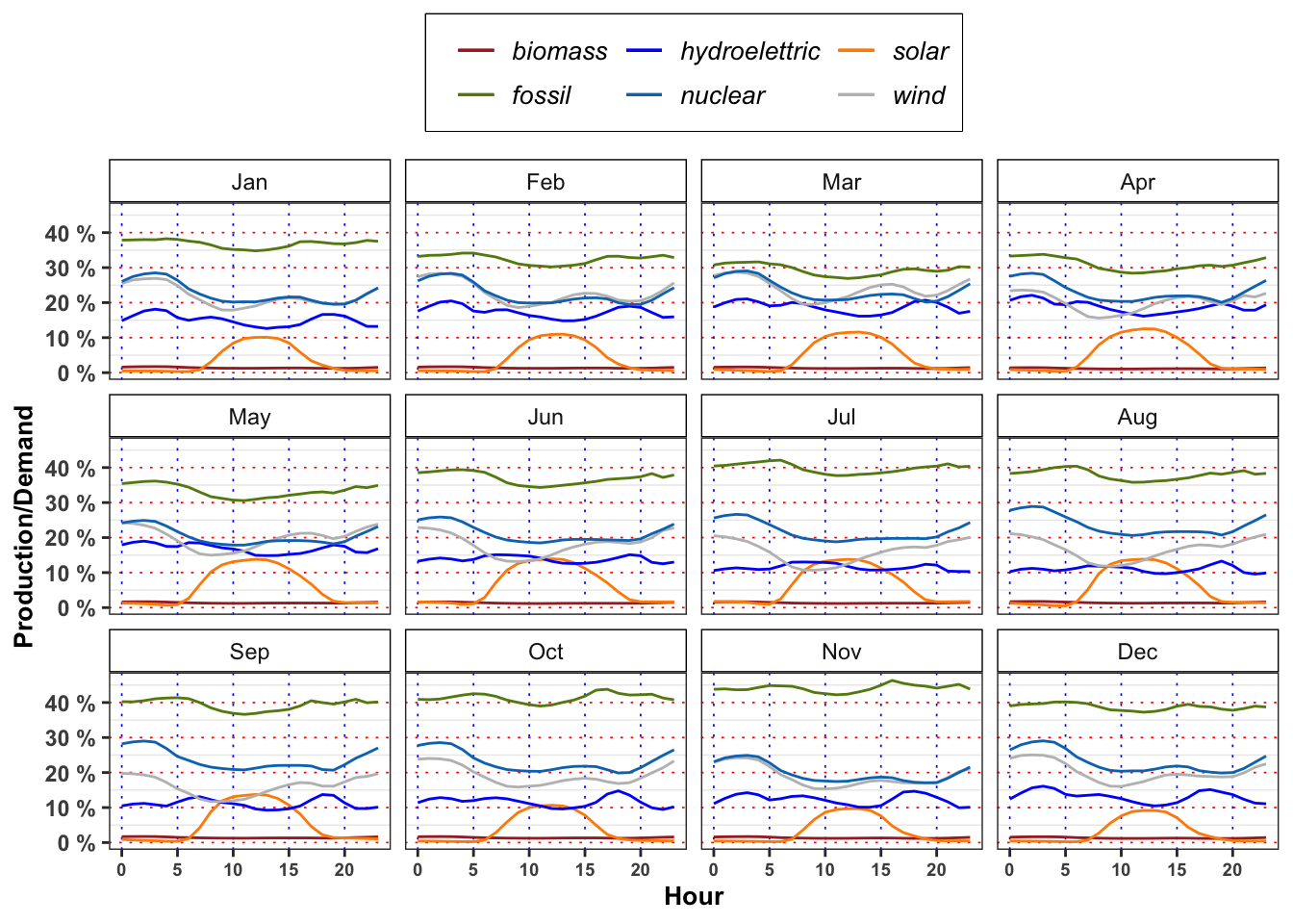
2.1.4 Task A.4
In mean, the demand satisfied by solar energy with respect to total demand is greater or lower with respect to the one satisfied by hydroelectric on 12:00 in March? In July, August and September at the same hour the situation changes? Answer, providing a possible explanation of the results obtained (max 200 words).
Code
df_A4 <- bind_rows(
   filter(df_A3, Month == "Mar" & Hour == 12),
   filter(df_A3, Month == "Jul" & Hour == 12),
   filter(df_A3, Month == "Aug" & Hour == 12),
   filter(df_A3, Month == "Sep" & Hour == 12)
)

df_A4 %>%
  mutate_if(is.numeric, ~.x*100) %>%
  mutate_if(is.numeric,  ~paste0(format(.x, digits = 3), " %"))  %>%
  mutate(demand = paste0(str_remove_all(demand, "\\%"), " MW"),
         Hour = paste0(as.numeric(str_remove_all(Hour, "\\%"))/100, ":00")) %>%
knitr::kable()| Month | Hour | biomass | solar | hydroelettric | wind | nuclear | fossil | demand |
|---|---|---|---|---|---|---|---|---|
| Mar | 12:00 | 1.19 % | 11.5 % | 16.7 % | 21.7 % | 20.9 % | 26.9 % | 3179217 MW |
| Jul | 12:00 | 1.19 % | 13.8 % | 11.8 % | 12.4 % | 19.1 % | 37.8 % | 3354479 MW |
| Aug | 12:00 | 1.28 % | 13.8 % | 10.3 % | 13.6 % | 20.9 % | 35.8 % | 3191764 MW |
| Sep | 12:00 | 1.28 % | 13.7 % | 9.6 % | 13.4 % | 21.3 % | 36.9 % | 3107519 MW |
2.1.5 Task A.5
Grouping the dataset firstly by season and hour (\(4 \times 24\) groups) and then by month and hour (\(12 \times 24\) groups) compute:
- Average electricity price
- Average ratio between total production and total demand, i.e.
prod/demand.
For both groups, answer to the following questions.
What is the meaning of a ratio between total production and total demand greater than 1? And greater than 1? Following the demand and supply law, what is the expected behavior of the price in such situations? Comment the results (max 200 words).
When the price reaches it’s minimum value? In such situation, does the ratio reach its maximum value? What happen when the prices reaches it’s maximum? Comment the results (max 200 words).
The minimum price for electricity by season and hour is reached, in mean, at 3:00 in all the seasons. Moreover, for all the seasons the ratio between production and demand is above 100% between 00:00 and 3:00 denoting a general excess of production with respect to the demand. Interestingly, when this ratio goes again above 100% again between 14:00 to 16:00 (except is summer) the price, in mean, reaches a relative minimum for the day.
On contrary the maximum price for the electricity, by season and hour is reached, in mean, at 19:00 except for Autumn (18:00). As expected, in the same period the production ratio reaches a minimum that for all the seasons is also a global minimum for the day.
In the monthly plots is highlighted the fact that is the drop in electricity price in 14:00 to 16:00 and the subsequent increase during the afternoon is smoothed going from May up to September.
Code
data %>%
  mutate(Month = lubridate::month(date_day, label = TRUE)) %>%
  mutate(prod = prod/demand) %>%
  group_by(Month, Hour) %>%
  summarise(prod = mean(prod, na.rm = TRUE)) %>%
  ggplot()+
  geom_line(aes(Hour, prod), color = "black")+
  geom_line(aes(Hour, 1), color = "red", linetype = "dashed")+
  facet_wrap(~Month)+
  theme_bw()+
  custom_theme+
  scale_y_continuous(breaks = seq(0, 1, 0.1),
                     labels = paste0(seq(0, 1, 0.1)*100, " %"))+
  labs(color = NULL, y = "Production/Demand")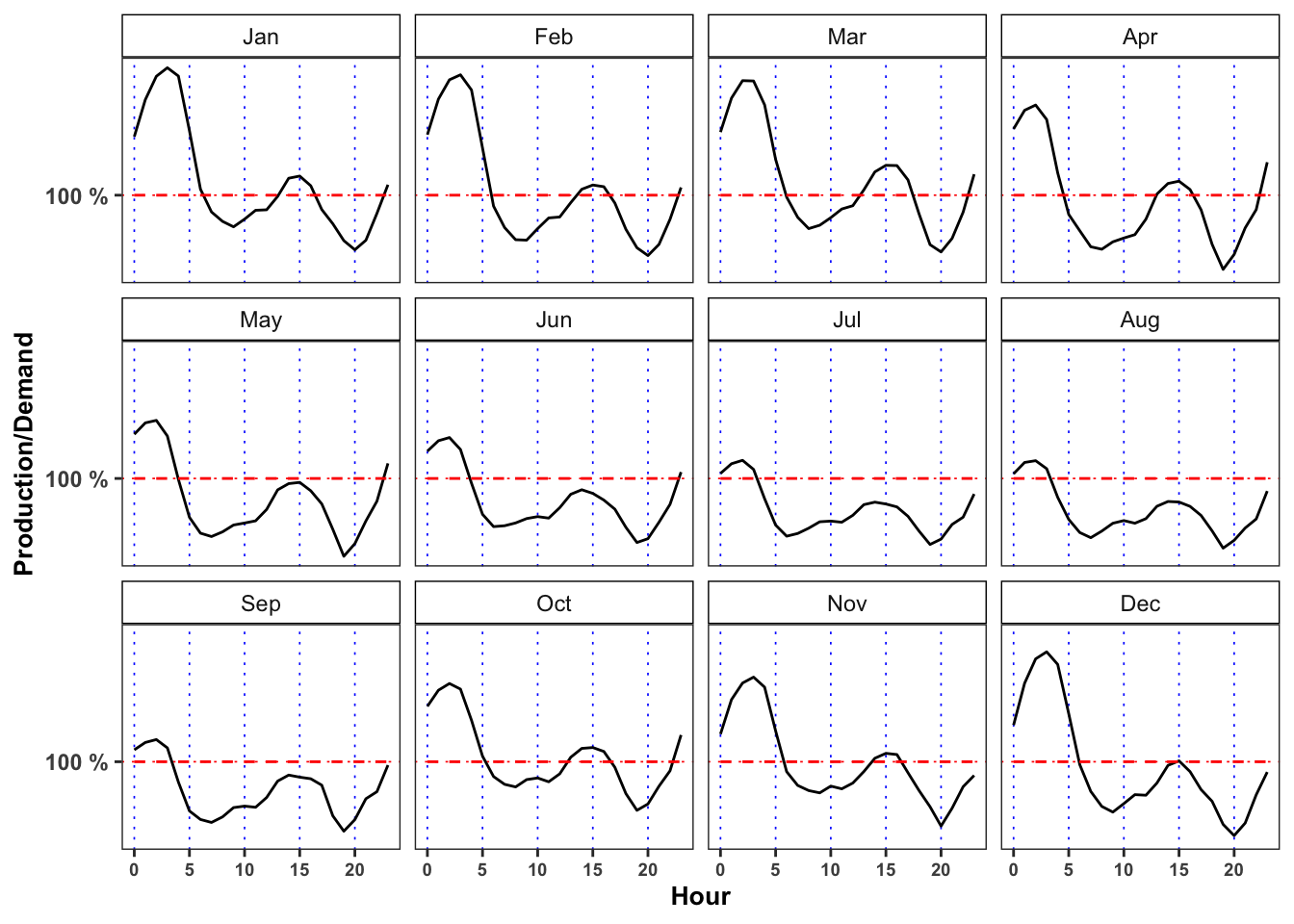
Code
data %>%
  mutate(Month = lubridate::month(date_day, label = TRUE)) %>%
  group_by(Month, Hour) %>%
  summarise(price = mean(price, na.rm = TRUE)) %>%
  ggplot()+
  geom_line(aes(Hour, price), color = "black")+
  facet_wrap(~Month)+
  theme_bw()+
  custom_theme+
  scale_y_continuous(breaks = seq(0, 100, 5),
                     labels = seq(0, 100, 5))+
  labs(color = NULL, y = "Price")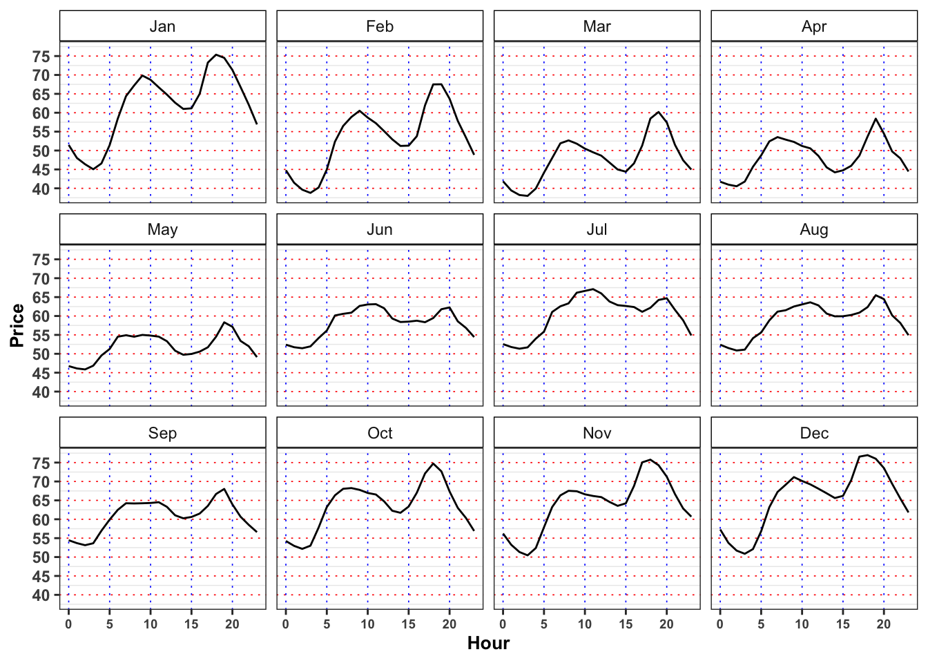
Code
data %>%
  mutate(prod = prod/demand) %>%
  group_by(Season, Hour) %>%
  summarise(prod = mean(prod, na.rm = TRUE)) %>%
  ggplot()+
  geom_line(aes(Hour, prod), color = "black")+
  geom_line(aes(Hour, 1), color = "red", linetype = "dashed")+
  facet_wrap(~Season)+
  theme_bw()+
  custom_theme+
  scale_x_continuous(breaks = seq(0, 24, 2))+
  scale_y_continuous(breaks = seq(0, 1, 0.1),
                     labels = paste0(seq(0, 1, 0.1)*100, " %"))+
  labs(color = NULL, y = "Production/Demand")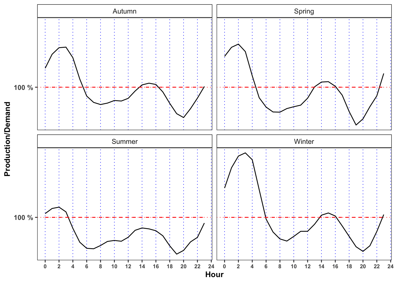
Code
data %>%
  group_by(Season, Hour) %>%
  summarise(price = mean(price, na.rm = TRUE)) %>%
  ggplot()+
  geom_line(aes(Hour, price))+
  geom_point(aes(Hour, price))+
  facet_wrap(~Season)+
  theme_bw()+
  custom_theme+
  scale_x_continuous(breaks = seq(0, 24, 2))+
  scale_y_continuous(breaks = seq(0, 100, 10))+
  labs(color = NULL, y = "Price (MW/h)")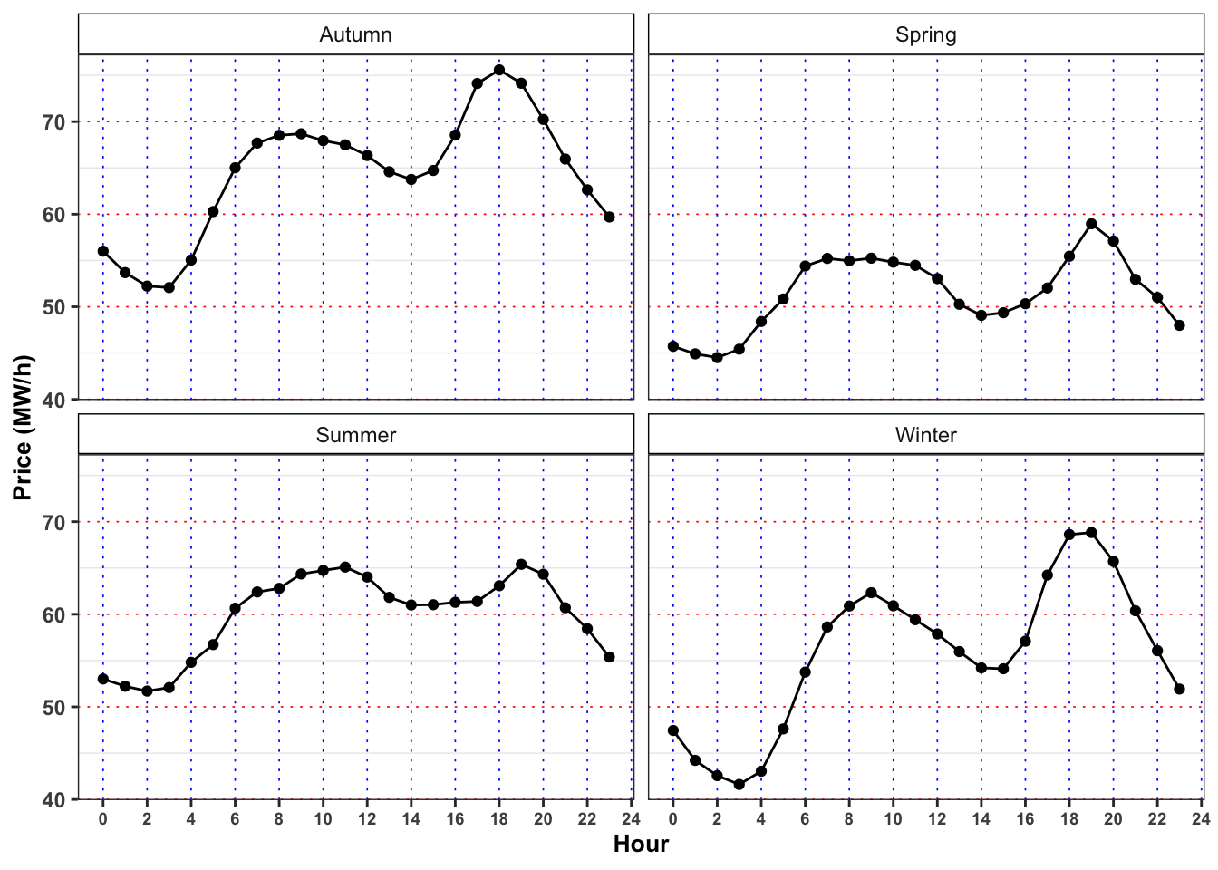
2.2 Problem B: Model hourly electricity price
2.2.1 Task B.1
Let’s define and estimate a model for the hourly electricity price. First of all, we have to define a seasonal function to remove deterministic patterns during the year and the day. Hence, we take into account a function of the form: \[ \begin{aligned} \bar{P}_t = p_0 + H(t) + M(t) \end{aligned} \] where \(H(t)\) stands for: \[ H(t) = \begin{cases} H_1 \quad \ \text{Hour} = 1 \\ H_2 \quad \ \text{Hour} = 2 \\ \vdots \\ H_{23} \quad \text{Hour} = 23 \\ \end{cases} \] and \(M(t)\) for: \[ M(t) = \begin{cases} M_2 \quad \ \text{Month} = \text{February} \\ \vdots \\ M_{12} \quad \text{Month} = \text{December} \\ \end{cases} \] It follows that, by construction, \(p_0\) captures the \(\text{Hour} = 0\) and \(\text{Month} = \text{January}\). Estimate the parameters of the models using OLS. Then, compute the seasonal price \(\bar{P}_t\) and the deseasonalized time series, i.e. \[ \tilde{P}_t = P_t - \bar{P}_t \] Plot \(\bar{P}_t\) and \(\tilde{P}_t\).
Seasonal model
# Model dataset
df_fit <- data
# Factor Variables
df_fit$Hour_ <- as.factor(df_fit$Hour)
df_fit$Month_ <- as.factor(df_fit$Month)
df_fit$Season_ <- as.factor(df_fit$Season)
# Seasonal model
seasonal_model <- lm(price ~ Hour_ + Month_, data = df_fit)
# Predicted seasonal mean
df_fit$price_bar <- predict(seasonal_model, newdata = df_fit)
# Fitted residuals
df_fit$price_tilde <- df_fit$price - df_fit$price_bar| r.squared | adj.r.squared | sigma | statistic | p.value | df | logLik | AIC | BIC | deviance | df.residual | nobs |
|---|---|---|---|---|---|---|---|---|---|---|---|
| 0.3178848 | 0.3172228 | 11.73688 | 480.1323 | 0 | 34 | -136089.5 | 272251.1 | 272555.8 | 4825399 | 35029 | 35064 |
| term | estimate | std.error | statistic | p.value |
|---|---|---|---|---|
| (Intercept) | 54.3007020 | 0.3696587 | 146.8941686 | 0.0000000 |
| Hour_1 | -1.7790349 | 0.4342528 | -4.0967725 | 0.0000420 |
| Hour_2 | -2.7812936 | 0.4342528 | -6.4047801 | 0.0000000 |
| Hour_3 | -2.7334839 | 0.4342528 | -6.2946835 | 0.0000000 |
| Hour_4 | -0.2004517 | 0.4342528 | -0.4616015 | 0.6443700 |
| Hour_5 | 3.3283436 | 0.4342528 | 7.6645301 | 0.0000000 |
| Hour_6 | 7.9087201 | 0.4342528 | 18.2122491 | 0.0000000 |
| Hour_7 | 10.4300068 | 0.4342528 | 24.0182838 | 0.0000000 |
| Hour_8 | 11.2295140 | 0.4342528 | 25.8593939 | 0.0000000 |
| Hour_9 | 12.0915127 | 0.4342528 | 27.8444096 | 0.0000000 |
| Hour_10 | 11.5433949 | 0.4342528 | 26.5822007 | 0.0000000 |
| Hour_11 | 11.0641205 | 0.4342528 | 25.4785246 | 0.0000000 |
| Hour_12 | 9.7660096 | 0.4342528 | 22.4892268 | 0.0000000 |
| Hour_13 | 7.6069815 | 0.4342528 | 17.5174038 | 0.0000000 |
| Hour_14 | 6.4553320 | 0.4342528 | 14.8653781 | 0.0000000 |
| Hour_15 | 6.7521629 | 0.4342528 | 15.5489222 | 0.0000000 |
| Hour_16 | 8.7482615 | 0.4342528 | 20.1455502 | 0.0000000 |
| Hour_17 | 12.3532717 | 0.4342528 | 28.4471900 | 0.0000000 |
| Hour_18 | 15.0938193 | 0.4342528 | 34.7581398 | 0.0000000 |
| Hour_19 | 16.2539220 | 0.4342528 | 37.4296313 | 0.0000000 |
| Hour_20 | 13.7690144 | 0.4342528 | 31.7073709 | 0.0000000 |
| Hour_21 | 9.4329911 | 0.4342528 | 21.7223498 | 0.0000000 |
| Hour_22 | 6.4771389 | 0.4342528 | 14.9155953 | 0.0000000 |
| Hour_23 | 3.1923340 | 0.4342528 | 7.3513264 | 0.0000000 |
| Month_2 | -8.3290915 | 0.3115812 | -26.7316899 | 0.0000000 |
| Month_3 | -13.7664987 | 0.3042645 | -45.2451707 | 0.0000000 |
| Month_4 | -13.3461258 | 0.3067895 | -43.5025441 | 0.0000000 |
| Month_5 | -9.7446337 | 0.3042645 | -32.0268521 | 0.0000000 |
| Month_6 | -3.4205772 | 0.3067895 | -11.1495884 | 0.0000000 |
| Month_7 | -1.2417608 | 0.3042645 | -4.0811886 | 0.0000449 |
| Month_8 | -2.6181552 | 0.3042645 | -8.6048663 | 0.0000000 |
| Month_9 | -0.7831501 | 0.3067895 | -2.5527274 | 0.0106925 |
| Month_10 | 1.8490054 | 0.3042645 | 6.0769674 | 0.0000000 |
| Month_11 | 2.2175860 | 0.3067895 | 7.2283624 | 0.0000000 |
| Month_12 | 3.7650571 | 0.3042645 | 12.3742904 | 0.0000000 |
Code
plot_seasonal <- df_fit %>%
  filter(Year == 2016 & Month %in% c(4:5) & Day %in% c(1:30))%>%
  ggplot()+
  geom_line(aes(date, price, color = "sample"))+
  geom_line(aes(date, price_bar, color = "seasonal"))+
  geom_line(aes(date, 0, color = "realized"), alpha = 0)+
  labs(x = NULL, y = TeX("$P_t$"), color = NULL)+
  scale_color_manual(values = c(sample = "orange", realized = "black", seasonal = "blue"),
                     labels = c(sample = "Sample", realized = "Realized residuals", seasonal = "Seasonal"))+
  theme_bw()+
  custom_theme
plot_eps <- df_fit %>%
  mutate(
    type = ifelse(Year == 2016 & Month %in% c(4:5) & Day %in% c(1:30), "col", "nocol")
  ) %>%
  ggplot()+
  geom_point(aes(date, price_tilde, color = type), size = 0.05)+
  labs(x = NULL, y = TeX("$\\tilde{P}_t$"), color = NULL)+
  scale_color_manual(values = c(col = "orange", nocol = "black"))+
  theme_bw()+
  custom_theme+
  theme(legend.position = "none")

gridExtra::grid.arrange(plot_seasonal, plot_eps, ncol = 1)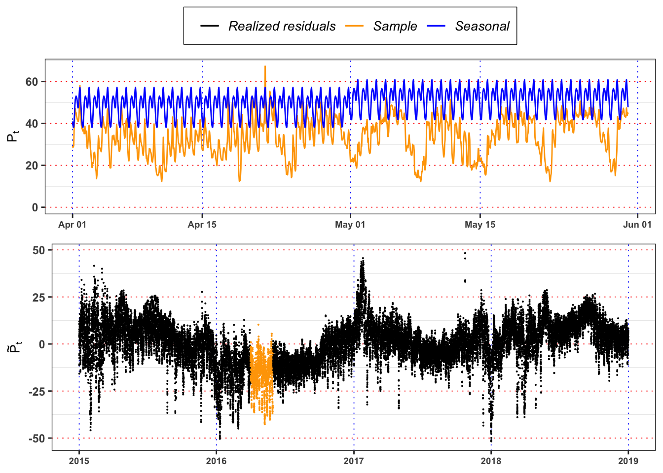
2.2.2 Task B.2
Estimate an autoregressive model (AR(1)) on the deseasonalized time series, i.e. \[ \begin{aligned} \tilde{P}_t = \phi \tilde{P}_{t-1} + \varepsilon_t \end{aligned} \] Is the estimated model stationary? Comment and justify your answer.
Hint: in order to answer consider the stationarity condition on the parameters.
Then, compute the fitted residuals \(\varepsilon_t\) and their standard deviation as: \[ \bar{\sigma} = \mathbb{S}d\{\varepsilon_t\} = \sqrt{\frac{1}{n-1}\sum_{t = 1}^n \varepsilon_t^2} \text{,} \] and the standardized residuals as \[ \bar{\varepsilon_t} = \frac{\varepsilon_t}{\bar{\sigma}} \text{.} \] Are \(\bar{\varepsilon_t}\) identically distributed? Answer with a formal statistics test with confidence level \(\alpha = 0.05\). (see for example see the two sample Kolmogorov-Smirnov test).
AR(1) model
# AR model
AR_model <- lm(price_tilde ~ I(lag(price_tilde, 1))-1, data = df_fit)
# Fitted values
df_fit$price_tilde_hat <- predict(AR_model, newdata = df_fit)
# Fitted residuals
df_fit$eps <- df_fit$price_tilde - df_fit$price_tilde_hat
# Estimated constant standard deviation
df_fit$sigma_bar <- sd(df_fit$eps, na.rm = TRUE)*sqrt(nrow(df_fit)/(nrow(df_fit)-1))
# Standardized residuals
df_fit$std_eps <- df_fit$eps/df_fit$sigma_bar
df_fit <- df_fit[-1,]| r.squared | adj.r.squared | sigma | logLik | AIC | BIC | deviance | df.residual | nobs |
|---|---|---|---|---|---|---|---|---|
| 0.9458574 | 0.9458559 | 2.729713 | -84961.89 | 169927.8 | 169944.7 | 261258.7 | 35062 | 35063 |
| term | estimate | std.error | statistic | p.value |
|---|---|---|---|---|
| $$\varphi$$ | 0.9725531 | 0.0012427 | 782.6393 | 0 |
Since 0.973 is less than 1 in absolute value the AR(1) is stationary. However, it is still present volatility clustering that makes the residuals non-stationary. The ADF-test, where \(H_0: \phi = 1\) (i.e. the process is non-stationary). If we reject \(H_0\) the process is stationary, otherwise it is explosive, i.e. non-stationary.
| statistic | p.value | parameter | method | lags | H0 |
|---|---|---|---|---|---|
| -10.66521 | 0.01 | 20 | Augmented Dickey-Fuller Test | 20 | Rejected (stationary) |
Code
plot_eps <- ggplot(df_fit)+
  geom_point(aes(date, eps, color = "eps"), size = 0.1, alpha = 0.4)+
  geom_line(aes(date, sigma_bar, color = "sigma"), size = 0.4)+
  geom_line(aes(date, -sigma_bar, color = "sigma"), size = 0.4)+
  geom_line(aes(date, 0, color = "std_eps"), alpha = 0)+
  labs(x = NULL, y = TeX("$\\epsilon_t$"), color = NULL)+
  custom_theme+
  scale_color_manual(values = c(eps = "black", sigma = "red", std_eps = "darkorange"),
                     labels = c(eps = TeX("$\\epsilon_t$"),
                                sigma = TeX("$\\pm\\bar{\\sigma}$"),
                                std_eps = TeX("$\\bar{\\epsilon}_t = \\frac{\\epsilon_t}{\\bar{\\sigma}}$")))+
  theme_bw()
plot_std_eps <- ggplot(df_fit)+
  geom_point(aes(date, std_eps), color = "orange", size = 0.1, alpha = 0.4)+
  geom_line(aes(date, sigma_bar), color = "red", size = 0.4)+
  geom_line(aes(date, -sigma_bar), color = "red", size = 0.4)+
  labs(x = NULL, y = TeX("$\\bar{\\epsilon}_t$"), color = NULL)+
  theme_bw()+
  custom_theme+
  theme(legend.position = "none")

gridExtra::grid.arrange(plot_eps, plot_std_eps)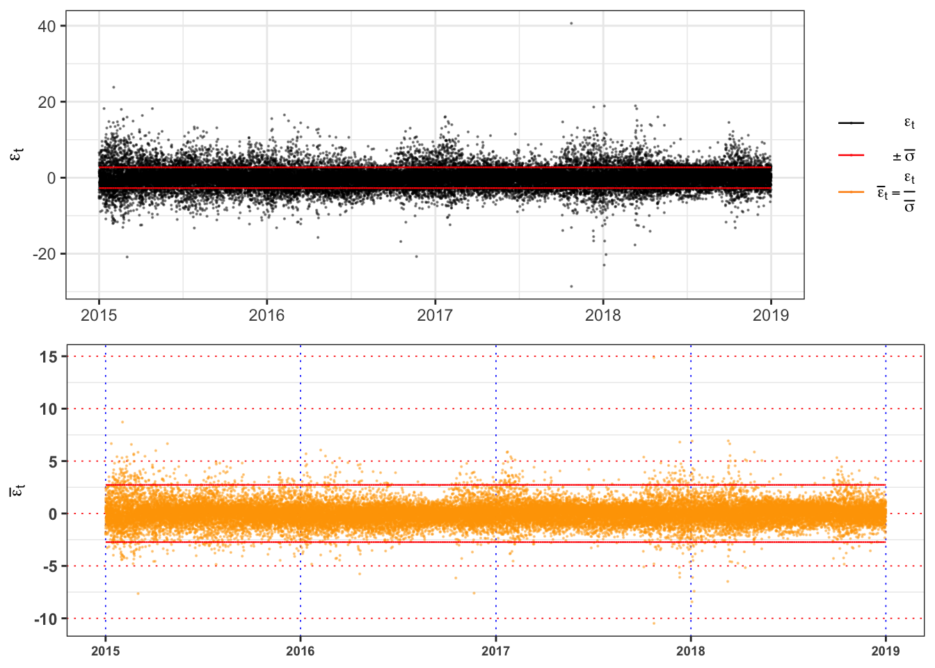
The graph above shows clearly that the standardized residuals presents volatility clusters, hence the time series of \(\bar{\epsilon}_t\) will be not identically distributed. A formal way to test it, is a two sample Kolmogorov-Smirnov.
KS-test on \(\bar{\epsilon}_t\)
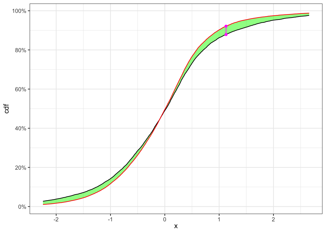
KS-test \(\bar{\epsilon}_t\)
kab <- solarr::ks.test(na.omit(df_fit$std_eps), ci = 0.01, seed = 1) %>%
  mutate_if(is.numeric, format, digits = 4, scientific = FALSE)
colnames(kab) <- c("$$\\textbf{Index split}$$", "$$\\alpha$$", "$$n_1$$", "$$n_2$$",
                   "$$KS_{n_1, n_2}$$", "$$\\textbf{Critical Level}$$", "$$H_0$$")
knitr::kable(kab, booktabs = TRUE, escape = FALSE, align = 'c')%>%
kableExtra::row_spec(0, color = "white", background = "green") | $$\textbf{Index split}$$ | $$\alpha$$ | $$n_1$$ | $$n_2$$ | $$KS_{n_1, n_2}$$ | $$\textbf{Critical Level}$$ | $$H_0$$ |
|---|---|---|---|---|---|---|
| 9310 | 1% | 9310 | 25753 | 0.04273 | 0.01968 | Rejected |
The null hypothesis of independence and identically distribution is rejected, hence we have to define a model for the conditional variance of the process.
2.2.3 Task B.3
A model for the conditional variance is the GARCH(p,q) model. Let’s consider a GARCH(1,2) model under the normality assumption., i.e. \[ \begin{aligned} & {}\varepsilon_t = \sigma_{t} u_t \\ & \sigma_{t}^2 = \omega + \alpha_1 \varepsilon_{t-1}^2 + \beta_1 \sigma_{t-1}^2 + \beta_2 \sigma_{t-2}^2 \\ & u_{t} \sim \; \mathcal{N}(0, 1) \end{aligned} \]
Is the estimated model stationary? Hint: in order to answer consider the stationarity condition on the parameters.
Compute the long-term variance under the GARCH(1,1) model, i.e. \(\mathbb{E}\{\sigma_t^2\}\), and compare it with the variance estimated in Task B.2 (i.e. \(\bar{\sigma}^2\)). Are the two variances similar? Comment the results.
Define the standardized GARCH residuals as: \[ u_t = \frac{\varepsilon_t}{\sigma_t} \] Are now the standardized residuals identically distributed? Answer using the same test used in Task B.2. Is the normality assumption satisfied on the fitted residuals? Answer with a formal test and a \(\alpha = 0.01\).
Hint: see for example see the Kolmogorov-Smirnov test.
GARCH(1,2) fit
# Variance specification
GARCH_spec <- rugarch::ugarchspec(
  variance.model = list(model = "sGARCH", garchOrder = c(1,2), external.regressors = NULL),
  mean.model = list(armaOrder = c(0,0), include.mean = FALSE), distribution.model = "norm")
# GARCH fitted model
GARCH_model <- rugarch::ugarchfit(data = df_fit$eps, spec = GARCH_spec, out.sample = 0)
# Fitted standard deviation
df_fit$sigma <- GARCH_model@fit$sigma
# Long-term standard deviation
df_fit$sigma_0 <- sqrt(GARCH_model@fit$coef[1]/(1-sum(GARCH_model@fit$coef[-1])))
# Fitted residuals
df_fit$ut <- df_fit$eps/df_fit$sigma
GARCH(1,2) table
kab <- tibble(
  params = c("$$\\omega$$", "$$\\alpha_1$$", "$$\\beta_1$$", "$$\\beta_2$$"),
  estimates = GARCH_model@fit$coef,
  se.coef = GARCH_model@fit$se.coef
) %>%
  mutate_if(is.numeric, format, digits = 3, scientific = FALSE)
knitr::kable(kab, booktabs = TRUE, escape = FALSE, align = 'c') %>%
kableExtra::row_spec(0, color = "white", background = "green") | params | estimates | se.coef |
|---|---|---|
| $$\omega$$ | 0.0407 | 0.0043341 |
| $$\alpha_1$$ | 0.0378 | 0.0008108 |
| $$\beta_1$$ | 0.2161 | 0.0000111 |
| $$\beta_2$$ | 0.7409 | 0.0000111 |
Since the sum \(\alpha_1 + \beta_1 + \beta_2 =\) 0.995 is less than 1 in absolute value the model is stationary.
Code
plot_std_eps <- ggplot(df_fit)+
  geom_point(aes(date, std_eps, color = "eps"), size = 0.1, alpha = 0.4)+
  geom_line(aes(date, sigma, color = "sigma"), size = 0.4)+
  geom_line(aes(date, -sigma, color = "sigma"), size = 0.4)+
  geom_line(aes(date, sigma_bar, color = "sigma_bar"), size = 0.4)+
  geom_line(aes(date, -sigma_bar, color = "sigma_bar"), size = 0.4)+
  geom_line(aes(date, 0, color = "std_eps"), alpha = 0)+
  geom_point(data = filter(df_fit, std_eps > sigma | std_eps < -sigma),
             aes(date, std_eps, color = "outliers"), size = 0.1)+
  labs(x = NULL, y = TeX("$\\bar{\\epsilon}_t$"), color = NULL)+
  scale_color_manual(values = c(eps = "black", outliers = "magenta",
                                sigma = "blue", sigma_bar = "red", std_eps = "darkorange"),
                     labels = c(eps = TeX("$\\bar{\\epsilon}_t = \\frac{\\epsilon_t}{\\bar{\\sigma}}$"),
                                sigma_bar = TeX("$\\pm\\bar{\\sigma}$"),
                                sigma = TeX("$\\pm\\sigma_t$"),
                                outliers = "Outliers",
                                std_eps = TeX("$u_t = \\frac{\\epsilon_t}{\\sigma_t}$")))+
  theme_bw()+
  custom_theme

plot_ut <- ggplot(df_fit)+
  geom_point(aes(date, ut), color = "orange", size = 0.1, alpha = 0.4)+
  geom_line(aes(date, sigma), color = "blue", size = 0.4)+
  geom_line(aes(date, -sigma), color = "blue", size = 0.4)+
  geom_line(aes(date, sigma_bar), color = "red", size = 0.4)+
  geom_line(aes(date, -sigma_bar), color = "red", size = 0.4)+
  geom_point(data = filter(df_fit, ut > sigma | ut < -sigma),
             aes(date, ut), color = "magenta", size = 0.1)+
  labs(x = NULL, y = TeX("$u_t$"), color = NULL)+
  theme_bw()+
  custom_theme+
  theme(legend.position = "none")

gridExtra::grid.arrange(plot_std_eps, plot_ut, heights = c(0.6, 0.4))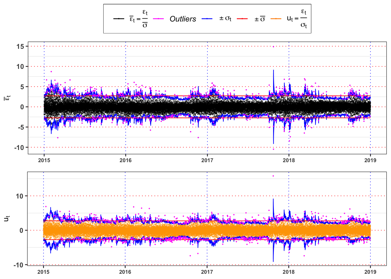
KS-test on \(u_t\)
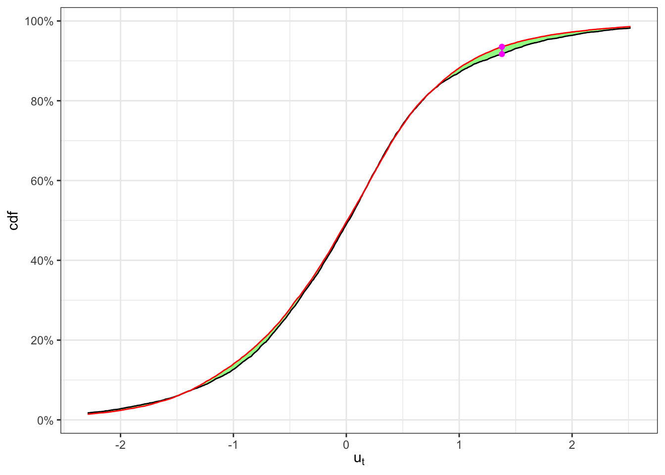
KS-test \(u_t\)
kab <- solarr::ks.test(na.omit(df_fit$ut), ci = 0.01, seed = 1) %>%
  mutate_if(is.numeric, format, digits = 4, scientific = FALSE)
colnames(kab) <- c("$$\\textbf{Index split}$$", "$$\\alpha$$", "$$n_1$$", "$$n_2$$",
                   "$$KS_{n_1, n_2}$$", "$$\\textbf{Critical Level}$$", "$$H_0$$")
knitr::kable(kab, booktabs = TRUE, escape = FALSE, align = 'c') %>%
kableExtra::row_spec(0, color = "white", background = "green") | $$\textbf{Index split}$$ | $$\alpha$$ | $$n_1$$ | $$n_2$$ | $$KS_{n_1, n_2}$$ | $$\textbf{Critical Level}$$ | $$H_0$$ |
|---|---|---|---|---|---|---|
| 9310 | 1% | 9310 | 25753 | 0.01827 | 0.01968 | Non-Rejected |
GARCH std deviation plot
ggplot(df_fit)+
  geom_line(aes(date, sigma, color = "sigma"), size = 0.3)+
  geom_line(aes(date, sigma_0, color = "sigma0"))+
  geom_line(aes(date, sigma_bar, color = "sigma_bar"))+
  geom_line(aes(date, 0, color = "std_eps"), alpha = 0)+
  labs(x = NULL, y = TeX("$\\sigma_t$"), color = NULL)+
  scale_y_continuous(limits = c(min(df_fit$sigma), max(df_fit$sigma)))+
  scale_color_manual(values = c(sigma = "black", sigma0 = "red", sigma_bar = "blue"),
                     labels = c(sigma = TeX("$\\sigma_t$"),
                                sigma0 = TeX("$\\sigma_0$"),
                                sigma_bar = TeX("$\\bar{\\sigma}$")))+
  theme_bw()+
  custom_theme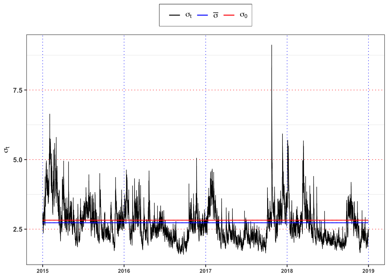
2.2.4 Task B.4
Let’s consider a Gaussian mixture model for the GARCH residuals, i.e. \[ u_t \sim B \cdot (\mu_{1} + \sigma_{1} Z_1) + (1-B) \cdot (\mu_{2} + \sigma_{2} Z_2) \]
where \(B \sim \text{Bernoulli}(p)\), while \(Z_1\) and \(Z_2\) are standard normal. All are assumed to be independent. Estimate the parameters \(\mu_{1}\), \(\mu_{2}\), \(\sigma_{1}\), \(\sigma_{2}\) and \(p\) with maximum likelihood (see here for an example). Consider the estimated parameters and give a possible interpretation of the two states, i.e. B = 1, B = 0.
Yearly Gaussian Mixture parameters
grid <- seq(-10, 10, 0.01)
init_params <- c(-mean(df_fit$ut), mean(df_fit$ut), 1, 1, 0.5)
opt <- solarr::fit_dnorm_mix(df_fit$ut, params = init_params)
params <- opt$par
names(params) <- c("$$\\mu_1$$", "$$\\mu_2$$", "$$\\sigma_1$$", "$$\\sigma_2$$", "$$p_1$$")
bind_rows(params) %>%
  bind_cols(p2 = 1 - params[5], log_lik = opt$value, mu_u = mean(df_fit$ut), sd_u = sd(df_fit$ut)) %>%
  mutate_if(is.numeric, format, digits = 4, scientific = FALSE) %>%
  knitr::kable(
    escape = FALSE,
    col.names = c("$$\\mu_1$$", "$$\\mu_2$$",
                  "$$\\sigma_1$$", "$$\\sigma_2$$", "$$p_1$$", "$$1-p_1$$",
"log-lik", "$$\\mathbb{E}\\{u_t\\}$$", "$$\\mathbb{S}d\\{u_t\\}$$"))| $$\mu_1$$ | $$\mu_2$$ | $$\sigma_1$$ | $$\sigma_2$$ | $$p_1$$ | $$1-p_1$$ | log-lik | $$\mathbb{E}\{u_t\}$$ | $$\mathbb{S}d\{u_t\}$$ |
|---|---|---|---|---|---|---|---|---|
| 0.04521 | -0.02346 | 1.489 | 0.6885 | 0.3015 | 0.6985 | -48452 | -0.002722 | 1 |
Yearly Gaussian Mixture vs Empirical densities
ggplot()+
  geom_density(data = df_fit, aes(ut), color = "black")+
  geom_line(aes(grid, 0, color = "ut"), alpha = 0)+
  geom_line(aes(grid, solarr::dnorm_mix(params)(grid), color = "nm"))+
  scale_color_manual(values = c(ut = "black", nm = "red"),
                     labels = c(ut = TeX("$u_t$"), nm = TeX("$GM(\\mu_1, \\mu_2, \\sigma_1, \\sigma_2, p)$")))+
  theme_bw()+
  custom_theme+
  labs(color = NULL)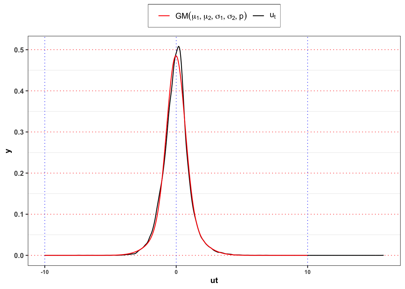
Yearly Gaussian Mixture vs Empirical monthly densities
pdf <- solarr::dnorm_mix(params)(grid)
df_grid <- tibble(Month = lubridate::month(1, label = TRUE), grid = grid, pdf = pdf)
for(i in 2:12){
  df_grid <- bind_rows(df_grid, mutate(df_grid, Month = lubridate::month(i, label = TRUE)))
}
df_fit %>%
  mutate(Month = lubridate::month(date, label = TRUE)) %>%
  ggplot()+
  geom_density(aes(ut), color = "red")+
  geom_line(data = df_grid, aes(grid, pdf), color = "blue")+
  facet_wrap(~Month)+
  scale_x_continuous(limits = c(-5, 5))+
  theme_bw()+
  custom_theme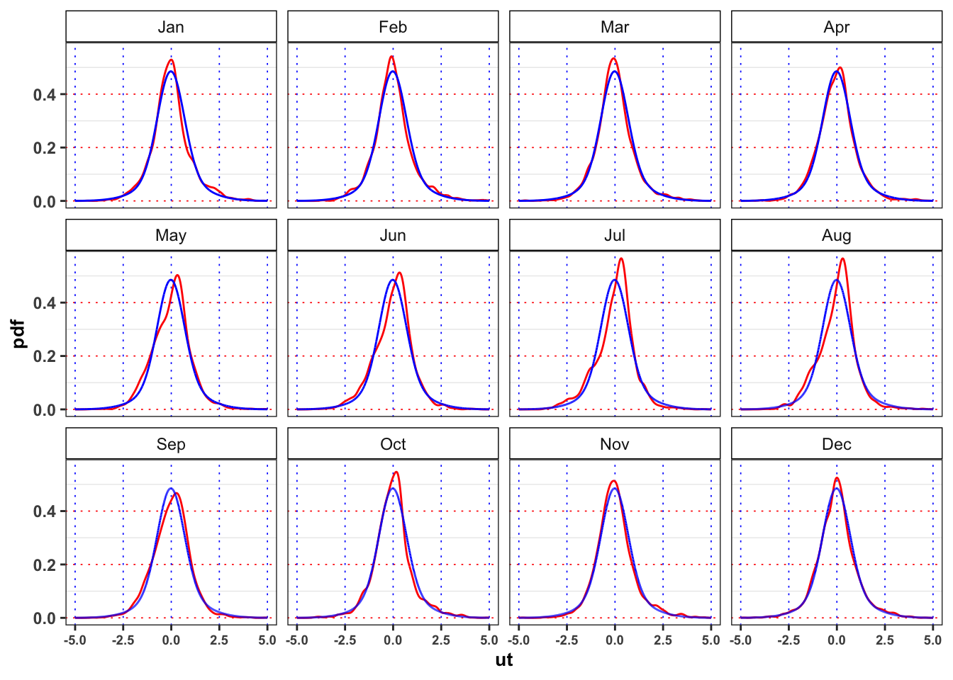
2.2.5 Task B.5
Let’s consider a monthly Gaussian mixture model for the GARCH residuals \(u_{t, m}\), where the index \(m = 1, \dots, 12\) denotes the \(m\)-month, i.e. \[ u_{t,m} \sim B_m \cdot Z_{m,1} + (1-B_m) \cdot Z_{m,2} \] where all the random variables, i.e. \[ \begin{aligned} {} & B_m \sim \text{Bernoulli}(p_m) \\ & Z_{m,1} = \mathcal{N}(\mu_{m,1},\sigma_{m,1}^2) \\ & Z_{m,2} = \mathcal{N}(\mu_{m,2},\sigma_{m,2}^2) \end{aligned} \] are assumed to be independent. Estimate the parameters for all the months with maximum likelihood.
Consider the following function as example. The main output should be a set of parameters. Due to the large number of estimates it is important to structure clearly the result that is necessary to produce many others estimates (e.g. VaR, simulations, …).
```{r}
function(x, date){

  # Define log-likelihood function
  log_lik <- function(params, x){
    # Parameters
    mu1 = params[1]
    mu2 = params[2]
    sd1 = params[3]
    sd2 = params[4]
    p = params[5]
    # Ensure that probability is in (0,1)
    if(p > 0.99 | p < 0.01 | sd1 < 0 | sd2 < 0){ s
      return(NA_integer_)
    }
    # Mixture density
    pdf_mix <- dnorm_mix(params)
    # Log-likelihood
    loss <- sum(pdf_mix(x, log = TRUE), na.rm = TRUE)
    return(loss)
  }

  # Extract the month
  M <- lubridate::month(date)
  # Initialize a dataset with all the variables
  data <- dplyr::tibble(Month = M, ut = x)
  # Fitting monthly routine
  NM_model <- list()
  for(i in 1:12){
    # Monthly data
    eps <- dplyr::filter(data, Month == i)$ut
    # Initial parameters
    init_params <- c(mu1 = -mean(eps), mu2 = mean(eps),
                     sd1 = sd(eps), sd2 = sd(eps), p = 0.5)
    # Optimal parameters (output: parameters and log-lik)
    nm <- optim(par = init_params, log_lik,
                x = eps, control = list(maxit = 500000, fnscale = -1))
    # Fitted parameters
    df_par <- dplyr::bind_rows(nm$par)
    df_par$p2 <- 1 - nm$par[5]
    df_par$log_lik <- nm$value
    # Rename variables
    colnames(df_par) <- c("mu1", "mu2", "sd1", "sd2", "p1", "p2")
    # Monthly data
    NM_model[[i]] <- dplyr::tibble(Month = i, df_par, nobs = length(eps))
  }
  # Reorder the components
  ## up: components with higher mean
  ## dw: components with lower mean
  NM_model <- dplyr::bind_rows(NM_model) %>%
    dplyr::mutate(
      # Greatest mean
      mu_up = dplyr::case_when(
        mu1 > mu2 ~ mu1,
        TRUE ~ mu2),
      sd_up = dplyr::case_when(
        mu1 > mu2 ~ sd1,
        TRUE ~ sd2),
     # Lowest mean
      mu_dw = dplyr::case_when(
        mu1 > mu2 ~ mu2,
        TRUE ~ mu1),
      sd_dw = dplyr::case_when(
        mu1 > mu2 ~ sd2,
        TRUE ~ sd1),
     # Probability of greatest
      p_up = dplyr::case_when(
        mu1 > mu2 ~ p1,
        TRUE ~ p2),
      p_dw = 1 -p_up
    )
  # Reorder the variables
  NM_model <- dplyr::select(NM_model, Month, mu_up, mu_dw, sd_up, sd_dw, p_up, p_dw, log_lik, nobs)
  return(NM_model)
}
```Monthly Gaussian Mixture parameters
NM_mixture <- solarr::fit_dnorm_mix.monthly(df_fit$ut, date = df_fit$date, match_moments = TRUE)
NM_mixture %>%
  mutate(Month = lubridate::month(Month, label = TRUE)) %>%
  select(Month:loss, e_x, v_x) %>%
  mutate_if(is.numeric, format, digits = 2, scientific = FALSE) %>%
  knitr::kable(
    escape = FALSE,
    col.names = c("Month", "$$\\mu_1$$", "$$\\mu_2$$",
                  "$$\\sigma_1$$", "$$\\sigma_2$$", "$$p_1$$", "$$1-p_1$$",
"log-lik", "$$\\mathbb{E}\\{u_t\\}$$", "$$\\mathbb{S}d\\{u_t\\}$$"))| Month | $$\mu_1$$ | $$\mu_2$$ | $$\sigma_1$$ | $$\sigma_2$$ | $$p_1$$ | $$1-p_1$$ | log-lik | $$\mathbb{E}\{u_t\}$$ | $$\mathbb{S}d\{u_t\}$$ |
|---|---|---|---|---|---|---|---|---|---|
| Jan | 0.1491 | -0.129 | 1.41 | 0.54 | 0.46 | 0.54 | -4177 | -0.00087 | 1.09 |
| Feb | 0.1506 | -0.118 | 1.40 | 0.56 | 0.43 | 0.57 | -3761 | -0.00184 | 1.05 |
| Mar | 0.2573 | -0.094 | 1.62 | 0.67 | 0.25 | 0.75 | -4067 | -0.00492 | 1.02 |
| Apr | 0.0069 | -0.040 | 0.77 | 1.73 | 0.83 | 0.17 | -3971 | -0.00112 | 1.00 |
| May | 0.3486 | -0.059 | 0.26 | 1.05 | 0.16 | 0.84 | -4097 | 0.00614 | 0.95 |
| Jun | 0.2982 | -0.131 | 0.39 | 1.12 | 0.30 | 0.70 | -3945 | -0.00369 | 0.96 |
| Jul | 0.2912 | -0.203 | 0.40 | 1.17 | 0.38 | 0.62 | -4021 | -0.01530 | 0.97 |
| Aug | 0.2965 | -0.136 | 0.35 | 1.10 | 0.31 | 0.69 | -3966 | -0.00302 | 0.91 |
| Sep | 0.0779 | -0.145 | 0.70 | 1.25 | 0.62 | 0.38 | -3916 | -0.00692 | 0.92 |
| Oct | 0.2648 | -0.083 | 1.79 | 0.65 | 0.24 | 0.76 | -4097 | -0.00096 | 1.11 |
| Nov | 0.3298 | -0.131 | 1.49 | 0.64 | 0.30 | 0.70 | -3913 | 0.00749 | 1.00 |
| Dec | 0.1011 | -0.071 | 1.43 | 0.64 | 0.37 | 0.63 | -4134 | -0.00735 | 1.02 |
Monthly Gaussian Mixture vs monthly empirical densities
df_grid <- tibble()
for(i in 1:12){
  params <- unlist(NM_mixture[i,][2:6])
  new_df <- tibble(Month = lubridate::month(i, label = TRUE), grid = grid, pdf = solarr::dnorm_mix(params)(grid))
  df_grid <- bind_rows(df_grid, new_df)
}
df_fit %>%
  mutate(Month = lubridate::month(date, label = TRUE)) %>%
  ggplot()+
  geom_density(aes(ut), color = "red")+
  geom_line(data = df_grid, aes(grid, pdf), color = "blue")+
  facet_wrap(~Month)+
  scale_x_continuous(limits = c(-5, 5))+
  theme_bw()+
  custom_theme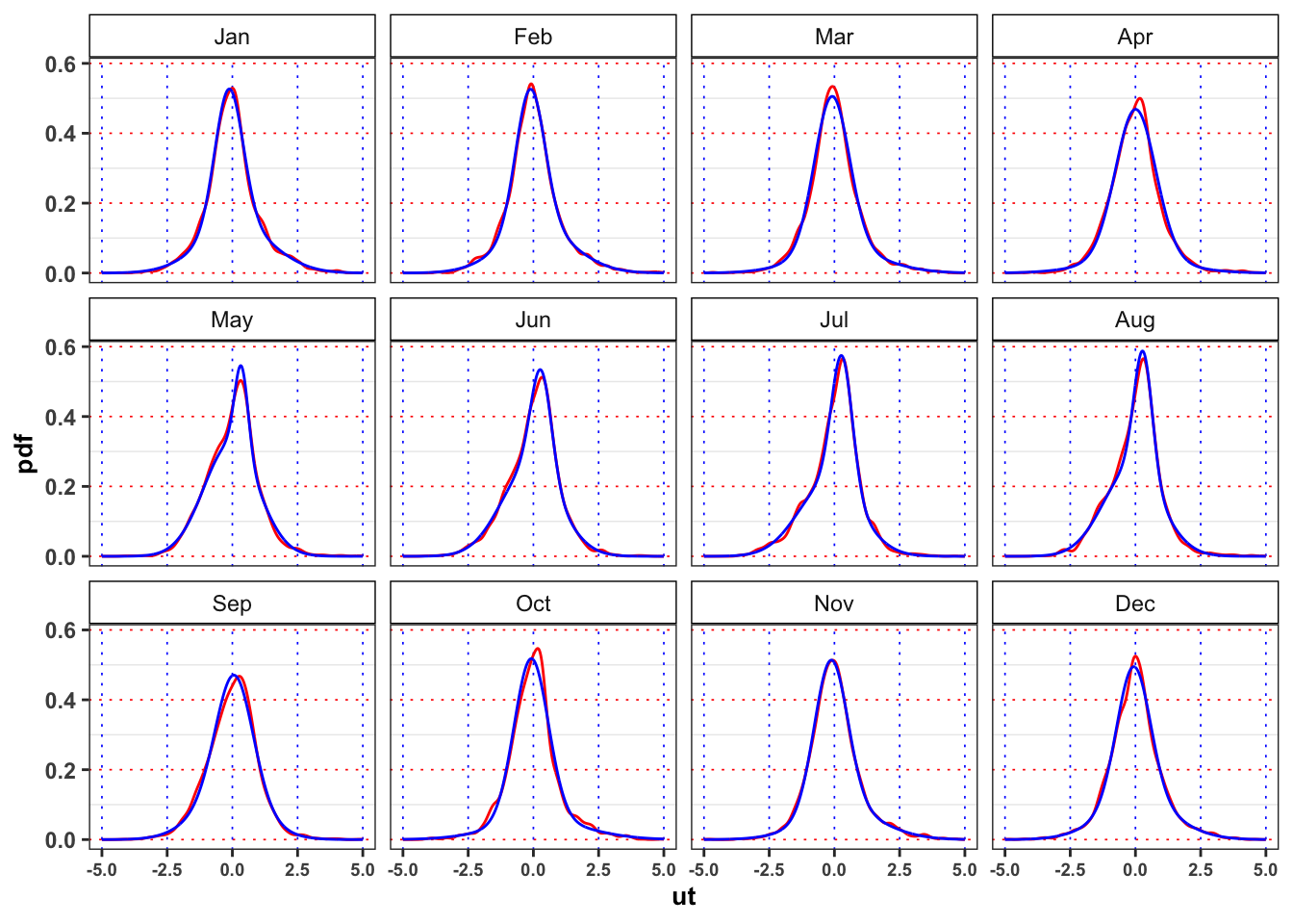
2.2.6 Task B.6
Let’s simulate hourly prices with the model and compare it with the empirical ones. You are free to choose between the basic Gaussian mixture and the monthly version. Then, consider the following two situations:
Projection A: You are
2017-06-28(known) and you want to simulate 100 trajectories for the price from2017-06-29up to2017-06-30(1 day, 24 hours).Projection B: You are in
2017-12-01(known) and you want to simulate 100 trajectories for the price from2017-12-02up to2017-12-31(29 days, 696 hours).
Be careful in simulations to always set a seed for reproducibility.
- The distribution of the residuals in the Projection A are close to the empirical distribution of the residuals in that month? The situation in Projection B changes? Is the model able to forecast the short term movements of the electricity price? Comment the results.
Hint 1: For a graphical comparison between densities you can plot the empirical histograms of \(u_t\) for the month \(m = 12\) (December) and the histograms of the simulated \(u_t\) for the same month.
Hint 2: Think about the fact that the aim of our model is to try to reproduce the distribution of the electricity prices and not to forecast it’s short term movements (potential omitted values could improve the model performances).
simulations
set.seed(1)
# Number of scenarios
j_bar <- 100
day_date <- seq.Date(as.Date("2017-06-29"), as.Date("2017-06-30"), 1)

# Extract year, month and day
Y <- lubridate::year(day_date)[1]
M <- lubridate::month(day_date)[1]
D <- lubridate::day(day_date)

# Datasets
df_emp <- filter(df_fit, Year == Y & Month == M & Day %in% D)
df_emp_plot <- filter(df_fit, Month == M & Day %in% D)
df_emp_plot <- right_join(select(df_emp, date, Month, Day, Hour),
                          select(df_emp_plot, -date), by = c("Month", "Day", "Hour"))
# Simulated scenarios
scenarios <- list()
for(j in 1:j_bar){
  # Initialize dataset
  df_sim <- df_emp
  # Simulated standard normal
  df_sim$ut <- rnorm(nrow(df_sim), mean = 0, sd = 1)
  df_sim$B <- 0
  # Single simulation
  for(i in 3:nrow(df_sim)){
    # Parameters
    # Extract month
    M_i <- lubridate::month(df_sim$date[i])
    # Gaussian mixture parameters
    NM <- unlist(NM_mixture[M_i, c(2:6)])
    # GARCH(1,1) parameters
    GARCH <- GARCH_model@fit$coef
    # AR(1) parameters
    phi <- AR_model$coefficients[1]
    # Simulation
    # Simulated binomial
    df_sim$B[i] <- rbinom(1, 1, prob = NM[5])
    # Simulated Gaussian mixture
    df_sim$ut[i] <- df_sim$B[i]*(NM[1] + NM[3]*df_sim$ut[i]) + (1-df_sim$B[i])*(NM[2] + NM[4]*df_sim$ut[i])
    # Simulated GARCH std. deviation
    df_sim$sigma[i] <- sqrt(GARCH[1] + GARCH[2]*df_sim$eps[i-1]^2 + GARCH[3]*df_sim$sigma[i-1]^2 + + GARCH[4]*df_sim$sigma[i-2]^2)
    # Simulated residuals
    df_sim$eps[i] <- df_sim$sigma[i]*df_sim$ut[i]
    # Simulated deseasonalized price
    df_sim$price_tilde[i] <- phi*df_sim$price_tilde[i-1] + df_sim$eps[i]
    # Seasonal mean
    # H <- as.factor(lubridate::hour(df_sim$date[i])))
    # S <- as.factor(solarr::detect_season(df_sim$date[i]))
    # df_sim$price_bar[i] <- predict(seasonal_model, newdata = tibble(Hour_ = H, Season_ = S))
    # Simulated price
    df_sim$price[i] <- df_sim$price_tilde[i] + df_sim$price_bar[i]
  }
  scenarios[[j]] <- dplyr::bind_cols(j = j, df_sim)
}

df_scenarios <- bind_rows(scenarios) %>%
  group_by(Hour) %>%
  mutate(e_price = mean(price))

plt_sim <-ggplot()+
  geom_line(data = df_scenarios, aes(date, price, group = j, color = "sim"), alpha = 0.3)+
  geom_line(data = df_scenarios, aes(date, e_price, group = j, color = "expected"))+
  geom_line(data = df_emp_plot, aes(date, price, group = Year, color = "year"))+
  geom_line(data = df_emp_plot, aes(date, price_bar, group = Year, color = "seasonal"), size = 1.2)+
  geom_line(data = df_emp, aes(date, price, color = "realized"), size = 1.2)+
  scale_color_manual(values = c(sim = "red", seasonal = "magenta", expected = "green",
                                realized = "purple", year = "black"),
                     labels = c(sim = "Simulated", seasonal = "Seasonal",
                                expected = "Expected",
                                realized = "Realized", year = "Other Years"))+
  theme_bw()+
  custom_theme+
  labs(color = NULL)

plt_hist <- ggplot()+
  geom_histogram(data = df_emp_plot, aes(ut, after_stat(density)),
                 color = "black", fill = "lightgray")+
  geom_density(data = df_sim, aes(ut), color = "red")+
  theme_bw()+
  labs(x = TeX("$u_t$"), y = NULL)+
  coord_flip()

gridExtra::grid.arrange(plt_sim, plt_hist, ncol = 2, widths = c(0.7, 0.3))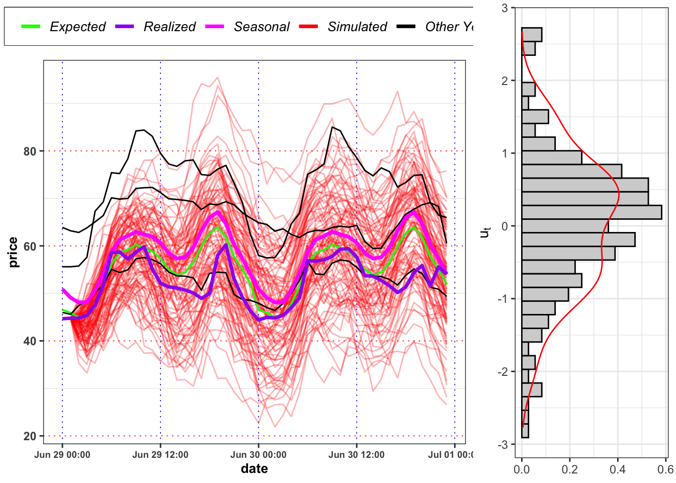
The projected price on 2017-06-30 23:00:00 is 53 Eur/MWh with a standard deviation of \(\pm\) 9.8 Eur/MWh,while the realized price was 54 Eur/MWh. Download
simulations
set.seed(1)
# Number of scenarios
j_bar <- 100
day_date <- seq.Date(as.Date("2015-12-01"), as.Date("2015-12-31"), 1)

# Extract year, month and day
Y <- lubridate::year(day_date)[1]
M <- lubridate::month(day_date)[1]
D <- lubridate::day(day_date)

# Datasets
df_emp <- filter(df_fit, Year == Y & Month == M & Day %in% D)
df_emp_plot <- filter(df_fit, Month == M & Day %in% D)
df_emp_plot <- right_join(select(df_emp, date, Month, Day, Hour),
                          select(df_emp_plot, -date), by = c("Month", "Day", "Hour"))
# Simulated scenarios
scenarios <- list()
for(j in 1:j_bar){
  # Initialize dataset
  df_sim <- df_emp
  # Simulated standard normal
  df_sim$ut <- rnorm(nrow(df_sim), mean = 0, sd = 1)
  df_sim$B <- 0
  # Single simulation
  for(i in 3:nrow(df_sim)){
    # Parameters
    # Extract month
    M_i <- lubridate::month(df_sim$date[i])
    # Gaussian mixture parameters
    NM <- unlist(NM_mixture[M_i, c(2:6)])
    # GARCH parameters
    GARCH <- GARCH_model@fit$coef
    # AR parameters
    phi <- AR_model$coefficients[1]
    # Simulation
    # Simulated binomial
    df_sim$B[i] <- rbinom(1, 1, prob = NM[5])
    # Simulated Gaussian mixture
    df_sim$ut[i] <- df_sim$B[i]*(NM[1] + NM[3]*df_sim$ut[i]) + (1-df_sim$B[i])*(NM[2] + NM[4]*df_sim$ut[i])
    # Simulated GARCH std. deviation
    df_sim$sigma[i] <- sqrt(GARCH[1] + GARCH[2]*df_sim$eps[i-1]^2 + GARCH[3]*df_sim$sigma[i-1]^2 + GARCH[4]*df_sim$sigma[i-2]^2)
    # Simulated residuals
    df_sim$eps[i] <- df_sim$sigma[i]*df_sim$ut[i]
    # Simulated deseasonalized price
    df_sim$price_tilde[i] <- phi*df_sim$price_tilde[i-1] + df_sim$eps[i]
    # Seasonal mean
    # H <- as.factor(lubridate::hour(df_sim$date[i])))
    # S <- as.factor(solarr::detect_season(df_sim$date[i]))
    # df_sim$price_bar[i] <- predict(seasonal_model, newdata = tibble(Hour_ = H, Season_ = S))
    # Simulated price
    df_sim$price[i] <- df_sim$price_tilde[i] + df_sim$price_bar[i]
  }
  scenarios[[j]] <- dplyr::bind_cols(j = j, df_sim)
}

df_scenarios <- bind_rows(scenarios) %>%
  group_by(Hour) %>%
  mutate(e_price = mean(price))

plt_sim <-ggplot()+
  geom_line(data = df_scenarios, aes(date, price, group = j, color = "sim"), alpha = 0.3)+
  geom_line(data = df_scenarios, aes(date, e_price, group = j, color = "expected"), size = 0.6)+
  geom_line(data = df_emp_plot, aes(date, price, group = Year, color = "year"))+
  geom_line(data = df_emp_plot, aes(date, price_bar, group = Year, color = "seasonal"), size = 0.6)+
  geom_line(data = df_emp, aes(date, price, color = "realized"), size = 0.6)+
  scale_color_manual(values = c(sim = "red", seasonal = "magenta", expected = "green",
                                realized = "purple", year = "black"),
                     labels = c(sim = "Simulated", seasonal = "Seasonal",
                                expected = "Expected",
                                realized = "Realized", year = "Other Years"))+
  theme_bw()+
  custom_theme+
  labs(color = NULL)

plt_hist <- ggplot()+
  geom_histogram(data = df_emp_plot, aes(ut, after_stat(density)),
                 color = "black", fill = "lightgray")+
  geom_density(data = df_sim, aes(ut), color = "red")+
  theme_bw()+
  custom_theme+
  labs(x = TeX("$u_t$"), y = NULL)+
  coord_flip()

gridExtra::grid.arrange(plt_sim, plt_hist, ncol = 2, widths = c(0.7, 0.3))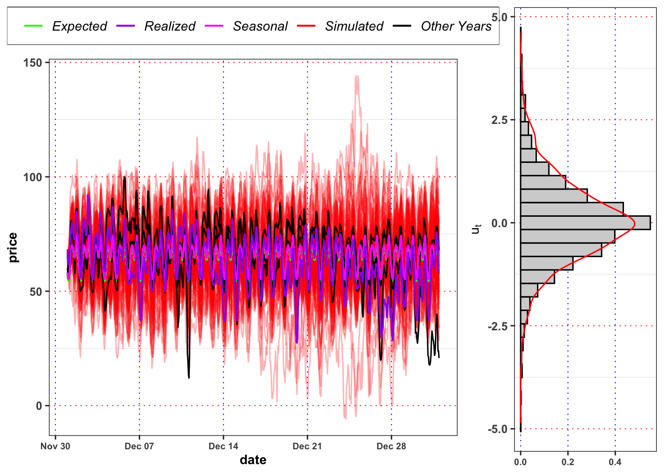
The projected price on 2015-12-31 23:00:00 is 62 Eur/MWh with a standard deviation of \(\pm\) 13 Eur/MWh,while the realized price was 58 Eur/MWh.
2.3 Potential extensions
- Propose a better model for electricity price, that can takes into account also external variables. You are free to chose an analytic or a Machine Learning approach.
- Propose a model for one of the natural variable available, for example see Peter Alaton and Stillberger (2002) for temperature or Alexandrinis and Zapranis (2013) for wind. Then, use the estimated model to price a weather derivative of your choice. In absence of a traded price, you can assume a market risk premium equal to zero and price the contract under \(\mathbb{P}\).
- Propose a complex derivative contract that can be used for hedging, the pricing procedure can be simplified if you use an approach based on copulas, see Bressan and Romagnoli (2021) as benchmark.
References
Citation
@online{sartini2024,
  author = {Sartini, Beniamino},
  title = {Hourly Energy Demand Generation and Weather},
  date = {2024-06-23},
  url = {https://greenfin.it/events/hourly-energy-demand-generation-and-weather.html},
  langid = {en}
}