Author

Affiliation

Beniamino Sartini

University of Bologna

1 Hourly energy demand generation and weather

library(tidyverse)
library(backports)
library(solarr)
library(latex2exp)

2 Description of the data

The dataset contains 4 years of electrical consumption, generation, pricing, and weather data for Spain. Consumption and generation data was retrieved from ENTSOE a public portal for Transmission Service Operator (TSO) data. Settlement prices were obtained from the Spanish TSO Red Electric España. Weather data was purchased as part of a personal project from the Open Weather API for the 5 largest cities in Spain. The original datasets can be downloaded from Kaggle. However, the dataset to be used for the project has been already pre-processed. The code used for preprocessing is in this github repository, while the dataset to be used can be downloaded here.

Tip 1: Variables description

• date: datetime index localized to CET.
• date_day: date without hour.
• city: reference city. (Valencia. Madrid, Bilbao,Barcelona, Seville)
• Year: number for the year.
• Month: number for the month.
• Day: number for the day in a month.
• Hour: reference hour of the day.

Energy variables

• fossil: energy produced with fossil sources: i.e. coal/lignite, natural gas, oil (MW).
• nuclear: energy produced with nuclear sources (MW).
• energy_other: other generation (MW).
• solar: solar generation (MW).
• biomass: biomass generation (MW).
• river: hydroeletric generation (MW).
• wind: wind generation (MW).
• energy_other_renewable: other renewable generation (MW).
• energy_waste: wasted generation (MW).
• pred_solar: forecasted solar generation (MW).
• pred_demand: forecasted electrical demand by TSO (MW).
• pred_price: forecasted day ahead electrical price by TSO (Eur/MWh).
• price: actual electrical price (Eur/MWh).
• demand: actual electrical demand (Eur/MWh).
• prod_tot: total electrical production (MW).
• prod_renewable: total renewable electrical production (MW).

Weather variables

• temp: mean temperature.
• temp_min: minimum temperature (degrees).
• temp_max: maximum temperature (degrees).
• pressure: pressure in (hPas).
• humidity: humidity in percentage.
• wind_speed: wind speed (m/s).
• wind_deg: wind direction.
• rain_1h: rain in last hour (mm).
• rain_3h: rain in last 3 hours (mm).
• snow_3h: show last 3 hours (mm).
• clouds_all: cloud cover in percentage.

dir_data <- "../grenfin-summer-school/data"
filepath <- file.path(dir_data, "data.csv")
data <- readr::read_csv(filepath, show_col_types = FALSE, progress = FALSE)
head(data) %>%
  knitr::kable(booktabs = TRUE ,escape = FALSE, align = 'c')%>%
  kableExtra::row_spec(0, color = "white", background = "green")

date	date_day	Year	Month	Day	Hour	Season	fossil	nuclear	energy_other	solar	biomass	river	energy_other_renewable	energy_waste	wind	pred_solar	pred_demand	pred_price	demand	price	prod	prod_renewable	temp	temp_min	temp_max	pressure	humidity	wind_speed	wind_deg	rain_1h	rain_3h	snow_3h	clouds_all
2014-12-31 23:00:00	2014-12-31	2014	12	31	23	Winter	10156	7096	43	49	447	3813	73	196	6378	17	26118	50.10	25385	65.41	27939	10687	-0.6585375	-5.825	8.475	1016.4	82.4	2.0	135.2	0	0	0	0
2015-01-01 00:00:00	2015-01-01	2015	1	1	0	Winter	10437	7096	43	50	449	3587	71	195	5890	16	24934	48.10	24382	64.92	27509	9976	-0.6373000	-5.825	8.475	1016.2	82.4	2.0	135.8	0	0	0	0
2015-01-01 01:00:00	2015-01-01	2015	1	1	1	Winter	9918	7099	43	50	448	3508	73	196	5461	8	23515	47.33	22734	64.48	26484	9467	-1.0508625	-6.964	8.136	1016.8	82.0	2.4	119.0	0	0	0	0
2015-01-01 02:00:00	2015-01-01	2015	1	1	2	Winter	8859	7098	43	50	438	3231	75	191	5238	2	22642	42.27	21286	59.32	24914	8957	-1.0605312	-6.964	8.136	1016.6	82.0	2.4	119.2	0	0	0	0
2015-01-01 03:00:00	2015-01-01	2015	1	1	3	Winter	8313	7097	43	42	428	3499	74	189	4935	9	21785	38.41	20264	56.04	24314	8904	-1.0041000	-6.964	8.136	1016.6	82.0	2.4	118.4	0	0	0	0
2015-01-01 04:00:00	2015-01-01	2015	1	1	4	Winter	7962	7098	43	34	410	3804	74	188	4618	4	21441	35.72	19905	53.63	23926	8866	-1.1260000	-7.708	7.317	1017.4	82.6	2.4	174.8	0	0	0	0

library(tidyverse)
library(backports)
library(solarr)
library(latex2exp)

3 Project

3.1 Problem A. Explorative analysis

Consider the data of the energy market in Spain and let’s examine the composition of the energy mix. At your disposal you have 5 sources that generate energy, i.e. 4 renewable (columns biomass, solar, river, wind) and 2 non-renewable (columns nuclear, fossil). The column demand denotes the amount of demanded electricity in MW, instead the column price denotes the actual price in $MW/h$. For simplicity, let’s denote with $E_t^{\mathbf{\ast }}$ the energy of the $\mathbf{\ast }$-th source, i.e.  $$E_t^{\mathbf{\ast }}=\{\begin{array}{l}{E}_t^b\mathbf{\ast }\to b=\text{biomass}\\ E_t^s\mathbf{\ast }\to s=\text{solar}\\ E_t^h\mathbf{\ast }\to h=\text{hydroelettric}\\ E_t^w\mathbf{\ast }\to w=\text{wind}\\ E_t^n\mathbf{\ast }\to n=\text{nuclear}\\ E_t^f\mathbf{\ast }\to f=\text{fossil}\end{array}$$ and the total energy demanded at time $t$ as $D_t$.

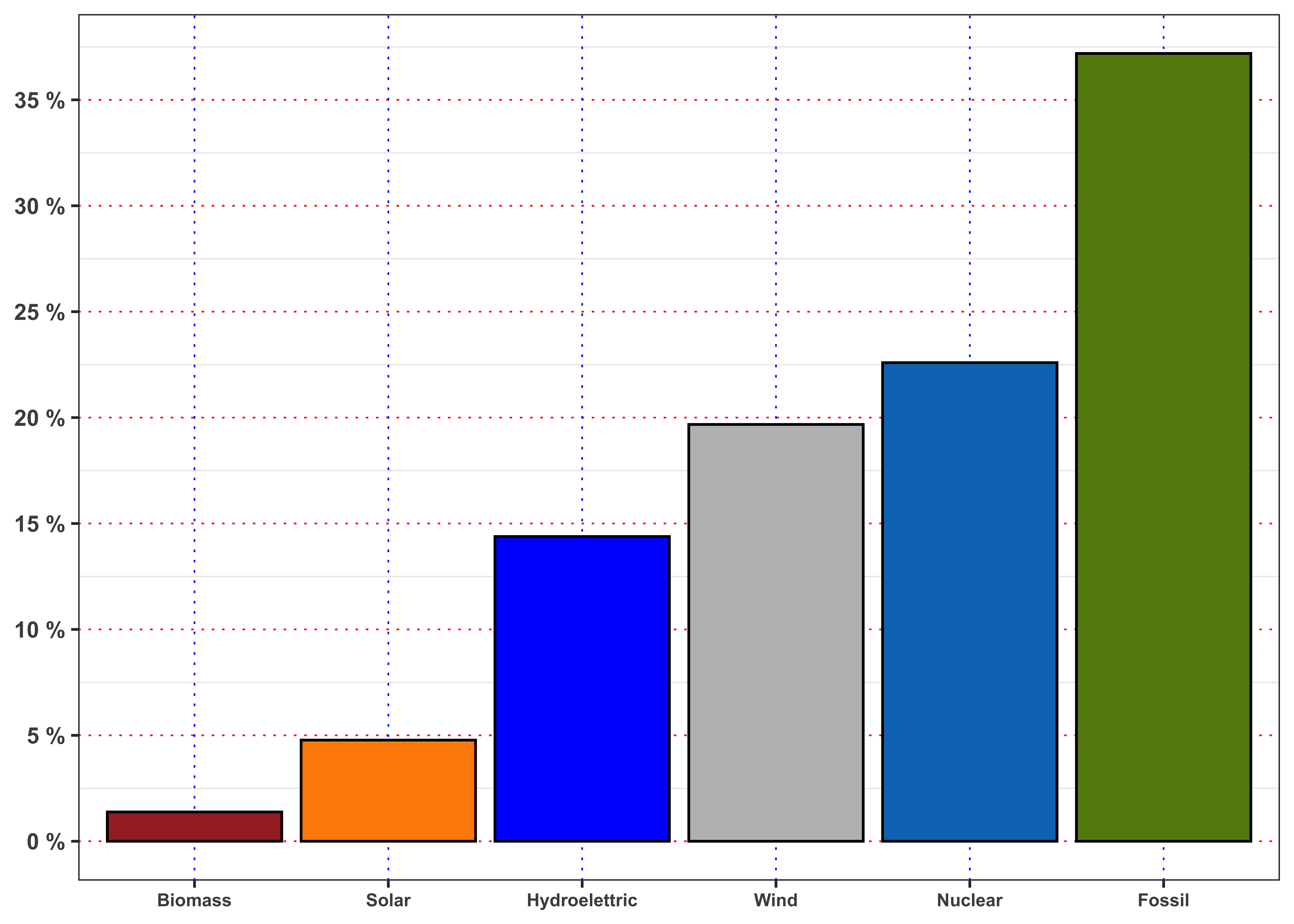
3.1.1 Task A.1

Compute the average between the energy produced from each source and the total demand, i.e.
$$\begin{array}{}\text{(1)}& R^{\mathbf{\ast }}=\frac{1}{n}\sum _{t=1}^n\frac{E_t^{\mathbf{\ast }}}{D_t}\end{array}$$

and normalize them, i.e. $R^{\mathbf{\ast }}/\sum R^{\mathbf{\ast }}$. Rank the 5 sources of energy by the percentage of demand satisfied in decreasing order and plot the values obtained with histograms.

Insert the password to see the solution of Task Task-A1

Solution A.1

var_levels <- c("biomass", "solar", "hydroelettric", "wind", "nuclear", "fossil")
var_labels <- c("Biomass", "Solar", "Hydroelettric", "Wind", "Nuclear", "Fossil")
# Compute the percentage ratio 
df_A1 <- data %>%
  dplyr::summarise(biomass = mean(biomass/demand),
                   solar = mean(solar/demand),
                   hydroelettric = mean(river/demand),
                   wind = mean(wind/demand),
                   nuclear = mean(nuclear/demand),
                   fossil = mean(fossil/demand))%>%
  tidyr::gather(key = "source", value = "perc")
# Categorical variable (plots purposes)
df_A1$id <- factor(df_A1$source, levels = var_levels, labels = var_labels)
# Normalize the percentages
df_A1$perc <- df_A1$perc/sum(df_A1$perc)

# Rank the sources 
vec_max <- df_A1$perc
names(vec_max) <- var_labels
vec_max_sort <- vec_max[order(vec_max, decreasing = TRUE)]

Download

df_A1 %>%
  ggplot()+
  geom_bar(aes(id, perc, fill = source), color = "black", stat = "identity")+
  theme_bw()+
  custom_theme+
  theme(legend.position = "none")+
  scale_fill_manual(values = c(fossil = "#65880f", nuclear = "#0477BF", biomass = "brown",
                               solar = "darkorange", hydroelettric = "blue", wind = "gray"))+
  scale_y_continuous(breaks = seq(0, 1, 0.05), 
                     labels = paste0(seq(0, 1, 0.05)*100, " %"))+
  labs(fill = NULL, x = NULL, y = NULL)

Figure 1: Mean percentage demand of energy satisfied by each source in Spain. Years 2015-2018.

The 1° source with respect to production/demand is Fossil (37.19%). The 2° source with respect to production/demand is Nuclear (22.59%). The 3° source with respect to production/demand is Wind (19.68%). The 4° source with respect to production/demand is Hydroelettric (14.39%). The 5° source with respect to production/demand is Solar (4.78%). The 6° source with respect to production/demand is Biomass (1.38%).

3.1.2 Task A.2

Aggregate the sources of energy in two groups:

1. Renewable: is given by the sum of solar, river, wind and biomass.
2. Non-renewable: is given by the sum of nuclear and fossil.

Then, compute the percentage of energy demand satisfied by each group. What is the percentage of energy satisfied by renewable sources? And by the fossil ones?

Repeat the computations, but filtering the data firstly only for year 2015 and then only for 2018. Are the percentage obtained different? Describe the result and explain if the transition to renewable energy is supported by data (to be supported the percentage of renewable energy should increase while percentage of fossil fuels should decrease.)

Insert the password to see the solution of Task Task-A2

Solution A.2

The percentage of demand satisfied by renewable sources is 40.22 %. Instead, the percentage of demand satisfied by fossil and nuclear sources is 59.78 %. The ratio of the fossil plus nuclear is 48.65 % bigger with respect to renewable sources.

# Percentage of demand by source in 2015
df_A2_2015 <- data %>%
  filter(Year == 2015) %>%
  summarise(biomass = mean(biomass/demand, na.rm = TRUE),
            solar = mean(solar/demand, na.rm = TRUE),
            river = mean(river/demand, na.rm = TRUE),
            wind = mean(wind/demand, na.rm = TRUE),
            nuclear = mean(nuclear/demand, na.rm = TRUE),
            fossil = mean(fossil/demand, na.rm = TRUE))%>%
  gather(key = "source", value = "perc") 
# Normalize 
df_A2_2015$perc <- df_A2_2015$perc/sum(df_A2_2015$perc)
# Categorical variable (plots purposes)
df_A2_2015$id <- factor(df_A2_2015$source, levels = var_levels, labels = var_labels)

# Percentage of demand by source in 2018
df_A2_2018 <- data %>%
  filter(Year == 2018) %>%
  summarise(biomass = mean(biomass/demand, na.rm = TRUE),
            solar = mean(solar/demand, na.rm = TRUE),
            river = mean(river/demand, na.rm = TRUE),
            wind = mean(wind/demand, na.rm = TRUE),
            nuclear = mean(nuclear/demand, na.rm = TRUE),
            fossil = mean(fossil/demand, na.rm = TRUE))%>%
  gather(key = "source", value = "perc")
# Normalize 
df_A2_2018$perc <- df_A2_2018$perc/sum(df_A2_2018$perc)
# Categorical variable (plots purposes)
df_A2_2018$id <- factor(df_A2_2018$source, levels = var_levels, labels = var_labels)

response <- paste0(
  "In 2015 the percentage of demand satisfied by renewable sources was ",
  round(sum(df_A2_2015$perc[1:4])*100, 3), " %, while in 2019 was ", 
  round(sum(df_A2_2018$perc[1:4])*100, 3), " %. ",
  "Hence, the dominance of renewable sources in this period increased by ",
  round((sum(df_A2_2018$perc[1:4])/sum(df_A2_2015$perc[1:4])-1)*100, 3), " %.",
  " Instead, in 2015 the percentage of demand satisfied by fossil and nuclear sources was ",
  round(sum(df_A2_2015$perc[5:6])*100, 3), " %, while in 2019 was ",
  round(sum(df_A2_2018$perc[5:6])*100, 3), " %. ",
  "Hence, the dominance of fossil sources in this period decreased by ",
  round((sum(df_A2_2018$perc[5:6])/sum(df_A2_2015$perc[5:6])-1)*100, 3), 
  " %. and the transition seems to be supported by data."
)

In 2015 the percentage of demand satisfied by renewable sources was 39.335 %, while in 2019 was 42.132 %. Hence, the dominance of renewable sources in this period increased by 7.111 %. Instead, in 2015 the percentage of demand satisfied by fossil and nuclear sources was 60.665 %, while in 2019 was 57.868 %. Hence, the dominance of fossil sources in this period decreased by -4.611 %. and the transition seems to be supported by data.

3.1.3 Task A.3

For each month, compute the mean percentage of demand of energy satisfied by the fossil sources. In order to compute $R_m^{\mathbf{\ast }}$ for the $m$-month, let’s denote with $n_m$ the number of day in that month, then: $$\begin{array}{}\text{(2)}& R_m^{\mathbf{\ast }}=\frac{1}{n_m}\sum _{t=1}^{n_m}\frac{E_t^{\mathbf{\ast }}}{D_t}=\frac{1}{n_m}\sum _{t=1}^{n_m}{R}_t^{\mathbf{\ast }}\end{array}$$

Compute also the maximum, minimum, median and standard deviation of $R_t^{\mathbf{\ast }}$ for each month. Repeat the computation for the others 4 sources of energy, i.e. nuclear, solar, river and wind. Which are the source with the lowest and the highest standard deviation in December? And in June? Comment the results obtained (max 200 words).

Insert the password to see the solution of Task Task-A3

Solution A.3

Fossil

df_fossil <- create_monthly_kable(data, target = "fossil")
df_fossil$kab

Percentage of energy demand satisfied by fossil.

Month	min	mean	meadian	max	sd
Jan	10.607 %	36.87 %	38.61 %	66.58 %	10.082 %
Feb	9.125 %	32.48 %	32.21 %	67.95 %	11.214 %
Mar	13.351 %	29.39 %	26.56 %	69.18 %	10.438 %
Apr	12.396 %	31.03 %	28.80 %	70.62 %	11.246 %
May	9.976 %	33.35 %	33.01 %	76.60 %	10.764 %
Jun	12.730 %	36.97 %	37.35 %	75.26 %	11.359 %
Jul	14.677 %	39.85 %	40.64 %	63.78 %	9.407 %
Aug	13.075 %	38.00 %	38.82 %	60.91 %	8.791 %
Sep	12.927 %	39.40 %	40.53 %	68.04 %	9.156 %
Oct	12.531 %	41.37 %	41.69 %	72.10 %	10.998 %
Nov	12.924 %	44.10 %	45.71 %	78.15 %	12.626 %
Dec	13.891 %	38.77 %	39.69 %	67.38 %	11.030 %

Nuclear

df_nuclear <- create_monthly_kable(data, target = "nuclear")
df_nuclear$kab

Percentage of energy demand satisfied by nuclear.

Month	min	mean	meadian	max	sd
Jan	12.271 %	22.74 %	21.86 %	39.22 %	4.498 %
Feb	11.660 %	22.56 %	21.77 %	38.42 %	4.655 %
Mar	13.040 %	23.46 %	22.74 %	36.57 %	4.504 %
Apr	12.624 %	23.13 %	22.65 %	37.64 %	4.906 %
May	4.999 %	20.40 %	19.98 %	37.59 %	3.990 %
Jun	12.569 %	21.17 %	20.67 %	37.76 %	4.381 %
Jul	12.390 %	21.65 %	21.09 %	34.93 %	3.956 %
Aug	12.780 %	23.61 %	23.08 %	34.00 %	4.113 %
Sep	13.929 %	23.65 %	22.98 %	35.29 %	4.348 %
Oct	14.127 %	23.09 %	22.54 %	35.85 %	4.503 %
Nov	0.000 %	19.82 %	19.25 %	33.38 %	4.343 %
Dec	13.425 %	23.08 %	22.31 %	39.37 %	5.219 %

Wind

df_wind <- create_monthly_kable(data, target = "wind")
df_wind$kab

Percentage of energy demand satisfied by wind.

Month	min	mean	meadian	max	sd
Jan	1.1883 %	21.80 %	20.39 %	62.26 %	11.609 %
Feb	1.5627 %	22.85 %	21.24 %	61.05 %	13.511 %
Mar	1.5243 %	24.03 %	23.67 %	64.02 %	12.726 %
Apr	1.8202 %	20.14 %	18.09 %	64.49 %	11.326 %
May	1.1022 %	19.88 %	17.45 %	57.96 %	11.555 %
Jun	1.0185 %	18.12 %	15.68 %	65.36 %	10.978 %
Jul	0.6918 %	15.96 %	14.27 %	59.08 %	9.259 %
Aug	0.7066 %	16.75 %	15.52 %	57.37 %	9.134 %
Sep	0.9261 %	16.05 %	13.60 %	56.38 %	10.383 %
Oct	0.7795 %	19.22 %	16.83 %	62.57 %	12.014 %
Nov	0.0000 %	18.93 %	16.16 %	69.16 %	12.136 %
Dec	1.6081 %	20.17 %	18.12 %	67.28 %	12.108 %

Hydroelettric

df_hydro <- create_monthly_kable(data, target = "river")
df_hydro$kab

Percentage of energy demand satisfied by hydroelettric.

Month	min	mean	meadian	max	sd
Jan	2.983 %	15.06 %	13.798 %	41.58 %	6.731 %
Feb	3.003 %	17.33 %	16.062 %	42.13 %	7.674 %
Mar	2.540 %	18.69 %	18.987 %	45.22 %	7.715 %
Apr	2.928 %	18.84 %	16.437 %	49.09 %	9.524 %
May	2.858 %	16.92 %	15.327 %	50.66 %	8.092 %
Jun	2.796 %	13.81 %	13.050 %	38.07 %	5.839 %
Jul	2.261 %	11.50 %	10.293 %	40.04 %	5.887 %
Aug	3.040 %	10.94 %	9.488 %	43.30 %	6.013 %
Sep	2.635 %	11.05 %	9.611 %	36.30 %	5.534 %
Oct	2.271 %	11.61 %	10.175 %	44.41 %	6.266 %
Nov	0.000 %	12.28 %	11.021 %	43.45 %	6.441 %
Dec	3.519 %	13.11 %	11.911 %	46.06 %	6.121 %

Solar

df_solar <- create_monthly_kable(data, target = "solar")
df_solar$kab

Percentage of energy demand satisfied by solar.

Month	min	mean	meadian	max	sd
Jan	0.024068 %	3.523 %	0.7840 %	25.38 %	4.830 %
Feb	0.006935 %	3.966 %	1.3321 %	22.70 %	5.080 %
Mar	0.018776 %	4.517 %	2.0257 %	21.22 %	5.345 %
Apr	0.009580 %	4.986 %	2.3468 %	21.88 %	5.572 %
May	0.008510 %	5.942 %	3.0158 %	22.48 %	5.939 %
Jun	0.011501 %	6.248 %	3.2706 %	22.03 %	5.761 %
Jul	0.008478 %	6.221 %	2.9958 %	23.40 %	5.726 %
Aug	0.009806 %	5.774 %	2.6587 %	21.32 %	5.825 %
Sep	0.017305 %	5.333 %	2.2467 %	23.02 %	5.875 %
Oct	0.007038 %	3.767 %	1.0721 %	21.75 %	4.974 %
Nov	0.000000 %	3.355 %	0.6537 %	18.63 %	4.619 %
Dec	0.008983 %	3.063 %	0.4059 %	19.26 %	4.386 %

Biomass

create_monthly_kable(data, target = "biomass")
## $data
## # A tibble: 12 × 6
##    Month     min   mean meadian    max      sd
##    <ord>   <dbl>  <dbl>   <dbl>  <dbl>   <dbl>
##  1 Jan   0.00732 0.0140  0.0138 0.0263 0.00350
##  2 Feb   0.00623 0.0139  0.0138 0.0274 0.00307
##  3 Mar   0.00476 0.0133  0.0131 0.0268 0.00406
##  4 Apr   0.00608 0.0119  0.0115 0.0282 0.00349
##  5 May   0       0.0139  0.0131 0.0272 0.00370
##  6 Jun   0.00675 0.0134  0.0128 0.0261 0.00348
##  7 Jul   0.00694 0.0136  0.0131 0.0272 0.00327
##  8 Aug   0.00527 0.0145  0.0137 0.0286 0.00378
##  9 Sep   0.00599 0.0142  0.0135 0.0281 0.00383
## 10 Oct   0.00543 0.0140  0.0131 0.0289 0.00403
## 11 Nov   0       0.0137  0.0130 0.0283 0.00372
## 12 Dec   0.00580 0.0134  0.0128 0.0280 0.00366
## 
## $kab
## 
## 
## |Month |min      |mean    |meadian |max     |sd       |
## |:-----|:--------|:-------|:-------|:-------|:--------|
## |Jan   |0.7321 % |1.404 % |1.383 % |2.630 % |0.3501 % |
## |Feb   |0.6226 % |1.394 % |1.380 % |2.741 % |0.3070 % |
## |Mar   |0.4760 % |1.334 % |1.306 % |2.680 % |0.4059 % |
## |Apr   |0.6078 % |1.191 % |1.147 % |2.819 % |0.3495 % |
## |May   |0.0000 % |1.394 % |1.308 % |2.718 % |0.3703 % |
## |Jun   |0.6752 % |1.344 % |1.277 % |2.614 % |0.3477 % |
## |Jul   |0.6938 % |1.365 % |1.305 % |2.719 % |0.3265 % |
## |Aug   |0.5274 % |1.447 % |1.373 % |2.859 % |0.3776 % |
## |Sep   |0.5987 % |1.424 % |1.348 % |2.809 % |0.3834 % |
## |Oct   |0.5433 % |1.404 % |1.314 % |2.890 % |0.4034 % |
## |Nov   |0.0000 % |1.372 % |1.298 % |2.830 % |0.3720 % |
## |Dec   |0.5796 % |1.339 % |1.284 % |2.801 % |0.3663 % |

sd_june <- c(fossil = filter(df_fossil$data, Month == "Jun")$sd,
             nuclear = filter(df_nuclear$data, Month == "Jun")$sd,
             wind = filter(df_wind$data, Month == "Jun")$sd,
             hydro = filter(df_hydro$data, Month == "Jun")$sd,
             solar = filter(df_solar$data, Month == "Jun")$sd)

sd_dec <- c(fossil = filter(df_fossil$data, Month == "Dec")$sd,
            nuclear = filter(df_nuclear$data, Month == "Dec")$sd,
            wind = filter(df_wind$data, Month == "Dec")$sd,
            hydro = filter(df_hydro$data, Month == "Dec")$sd,
            solar = filter(df_solar$data, Month == "Dec")$sd)

min_sd_jun <- sd_june[order(sd_june, decreasing = FALSE)][1]
min_sd_dec <- sd_dec[order(sd_dec, decreasing = FALSE)][1]
max_sd_jun <- sd_june[order(sd_june, decreasing = FALSE)][length(sd_june)]
max_sd_dec <- sd_dec[order(sd_dec, decreasing = FALSE)][length(sd_dec)]

The nuclear energy has the lowest standard deviation of percentage demand satisfied in June with a standard deviation of 4.4 %. The maximum standard deviation is from fossil with 11 %.

Instead the solar energy has the lowest standard deviation of percentage demand satisfied in December with a standard deviation of 4.4 %. The maximum standard deviation is from wind with 12 %.

Download

df_A3 <- data %>%
  mutate(Month = lubridate::month(date_day, label = TRUE)) %>%
  group_by(Month, Hour) %>%
  summarise(biomass = mean(biomass/demand, na.rm = TRUE), 
            solar = mean(solar/demand, na.rm = TRUE), 
            hydroelettric = mean(river/demand, na.rm = TRUE),
            wind = mean(wind/demand, na.rm = TRUE),
            nuclear = mean(nuclear/demand, na.rm = TRUE),
            fossil = mean(fossil/demand, na.rm = TRUE),
            demand = mean(demand, na.rm = TRUE))
 
ggplot(df_A3)+
    geom_line(aes(Hour, biomass, color = "biomass"))+
    geom_line(aes(Hour, solar, color = "solar"))+
    geom_line(aes(Hour, hydroelettric, color = "hydroelettric"))+
    geom_line(aes(Hour, wind, color = "wind"))+
    geom_line(aes(Hour, nuclear, color = "nuclear"))+
    geom_line(aes(Hour, fossil, color = "fossil"))+
    facet_wrap(~Month)+
    theme_bw()+
    custom_theme+
    scale_color_manual(values = c(fossil = "#65880f", nuclear = "#0477BF", biomass = "brown",
                                  solar = "darkorange", hydroelettric = "blue", wind = "gray"))+
    scale_y_continuous(breaks = seq(0, 1, 0.1), 
                       labels = paste0(seq(0, 1, 0.1)*100, " %"))+
    labs(color = NULL, y = "Production/Demand")

Figure 2: Mean percentage demand of energy satisfied by each source in Spain by hour and month. Years 2015-2018.

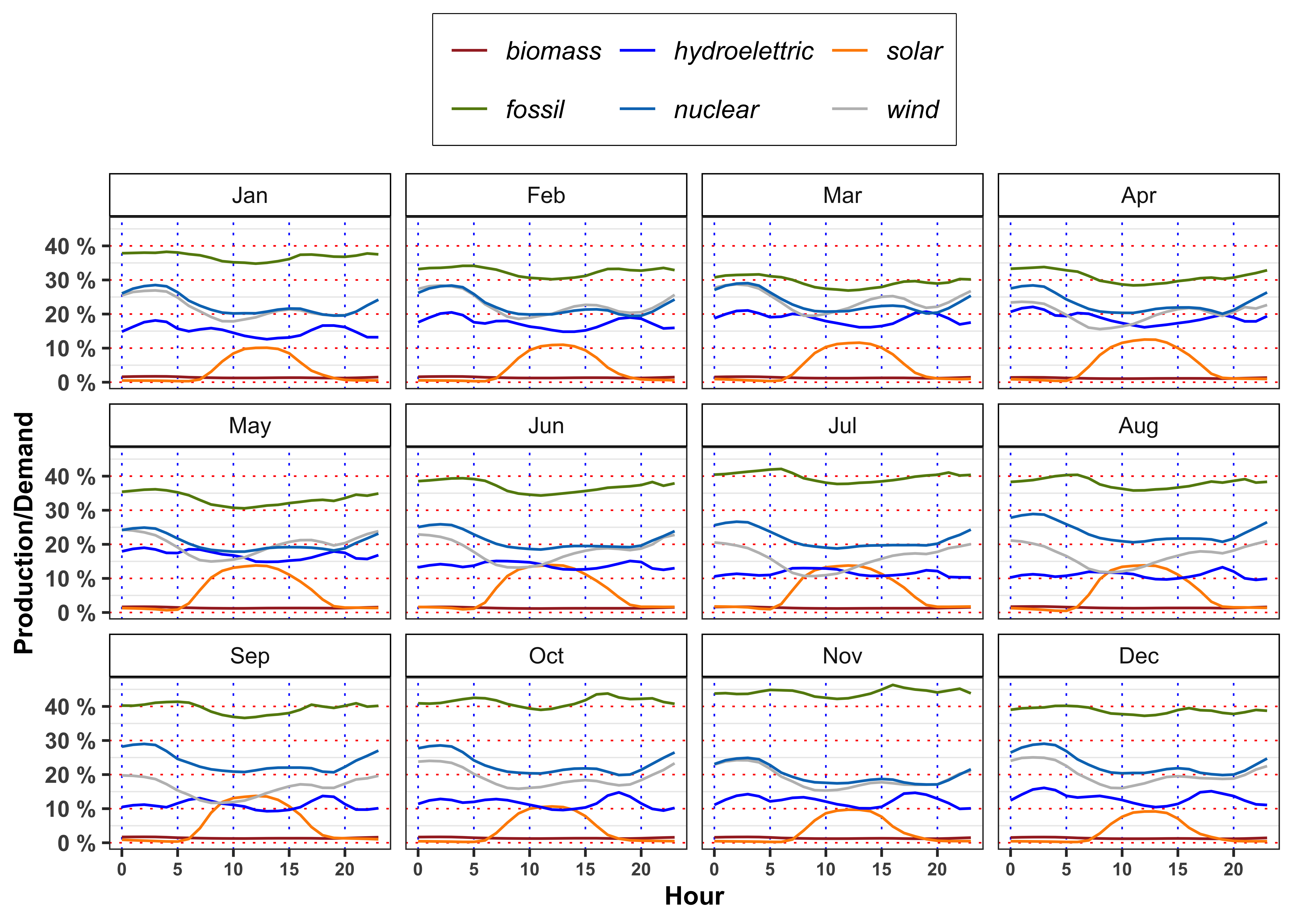
3.1.4 Task A.4

In mean, the demand satisfied by solar energy with respect to total demand is greater or lower with respect to the one satisfied by hydroelectric on 12:00 in March? In July, August and September at the same hour the situation changes? Answer, providing a possible explanation of the results obtained (max 200 words).

Insert the password to see the solution of Task Task-A4

Solution A.4

df_A4 <- bind_rows(
   filter(df_A3, Month == "Mar" & Hour == 12),
   filter(df_A3, Month == "Jul" & Hour == 12),
   filter(df_A3, Month == "Aug" & Hour == 12),
   filter(df_A3, Month == "Sep" & Hour == 12)
)

df_A4 %>%
  mutate_if(is.numeric, ~.x*100) %>%
  mutate_if(is.numeric,  ~paste0(format(.x, digits = 3), " %"))  %>%
  mutate(demand = paste0(str_remove_all(demand, "\\%"), " MW"),
         Hour = paste0(as.numeric(str_remove_all(Hour, "\\%"))/100, ":00")) %>%
  knitr::kable()

Month	Hour	biomass	solar	hydroelettric	wind	nuclear	fossil	demand
Mar	12:00	1.19 %	11.5 %	16.7 %	21.7 %	20.9 %	26.9 %	3179217 MW
Jul	12:00	1.19 %	13.8 %	11.8 %	12.4 %	19.1 %	37.8 %	3354479 MW
Aug	12:00	1.28 %	13.8 %	10.3 %	13.6 %	20.9 %	35.8 %	3191764 MW
Sep	12:00	1.28 %	13.7 %	9.6 %	13.4 %	21.3 %	36.9 %	3107519 MW

# More hydroelettric on March at 12:00
# More solar on Jul, Aug, Sep at 12:00
# Interpret: more sun less water in Summer. 

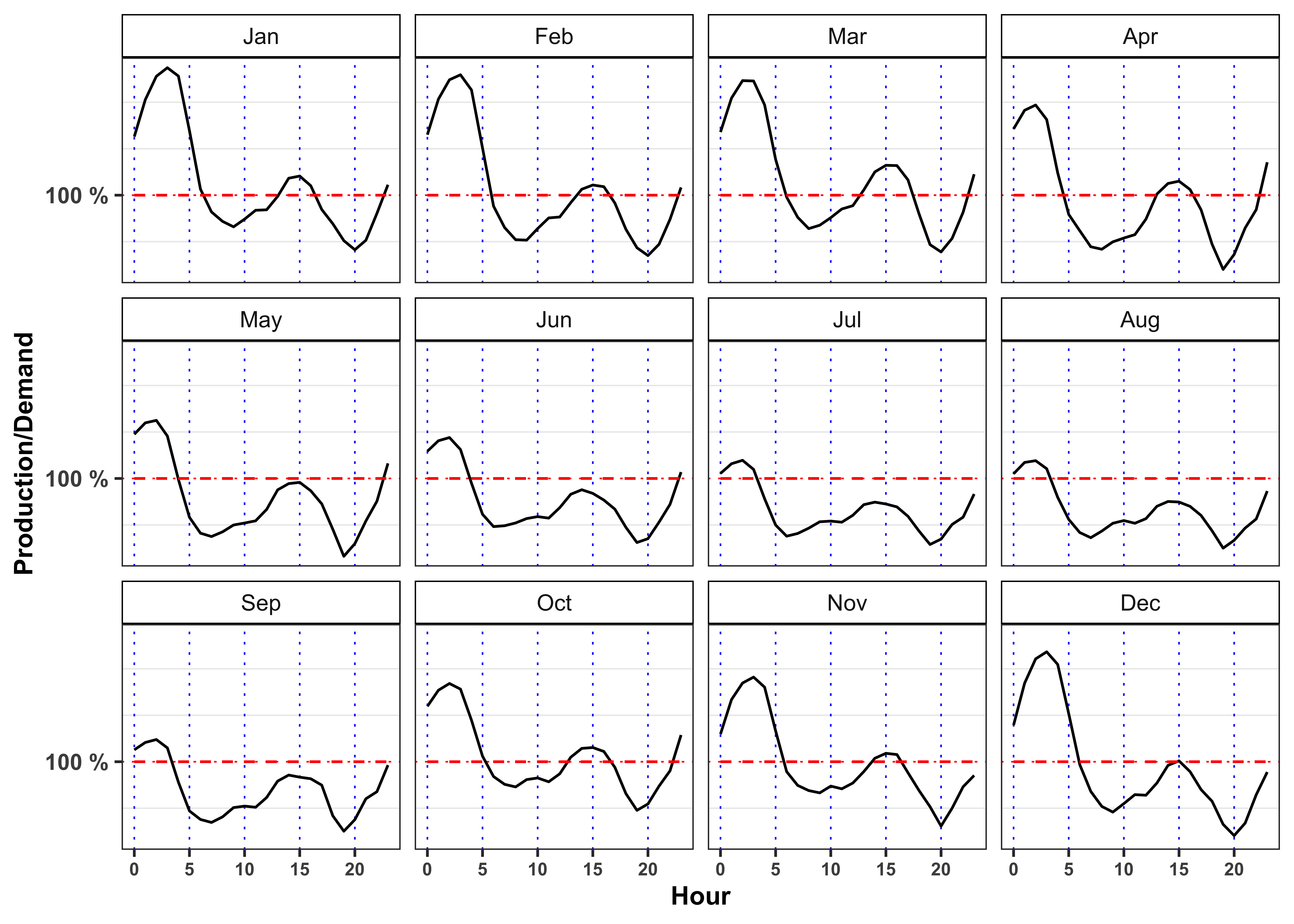
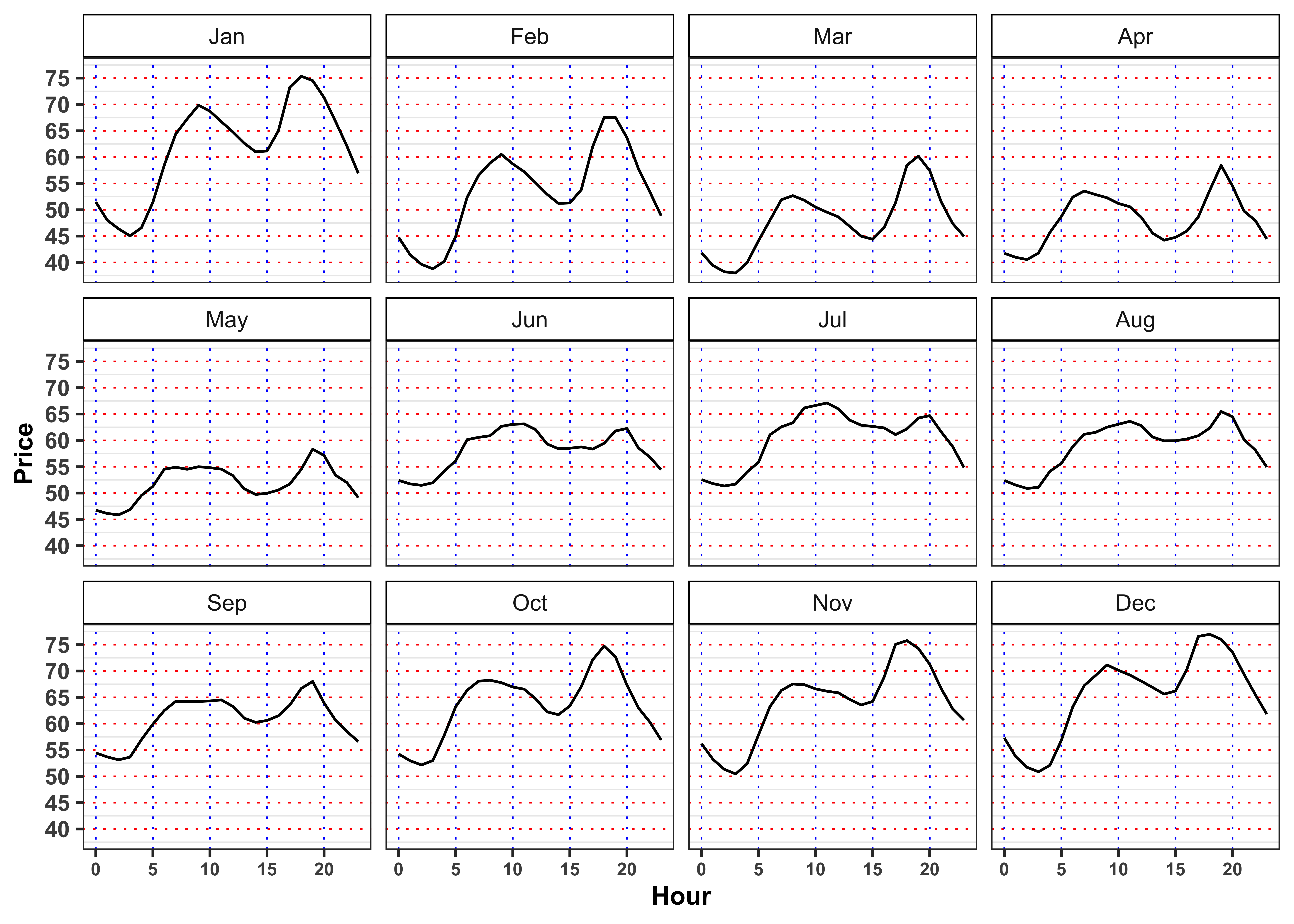
3.1.5 Task A.5

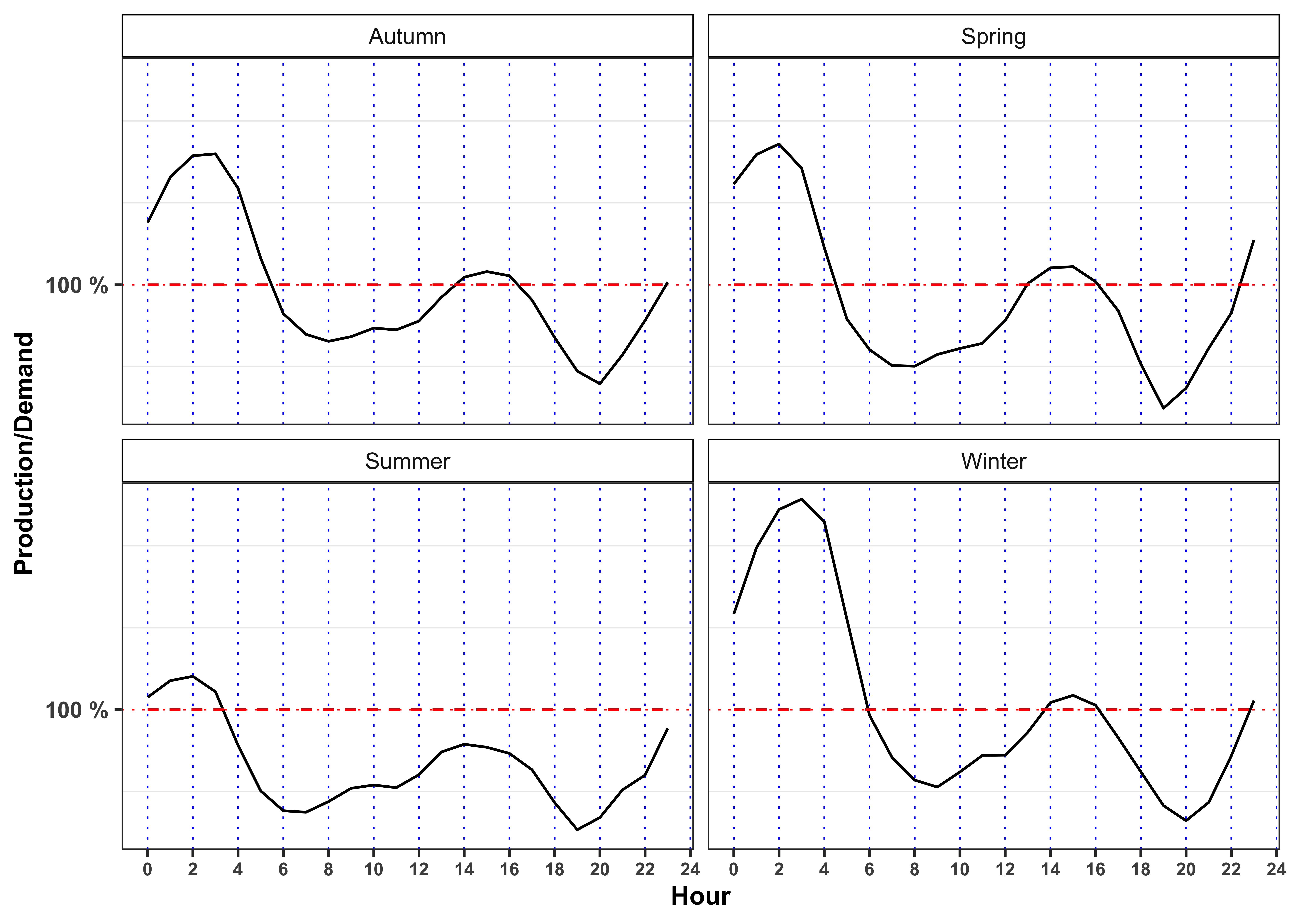
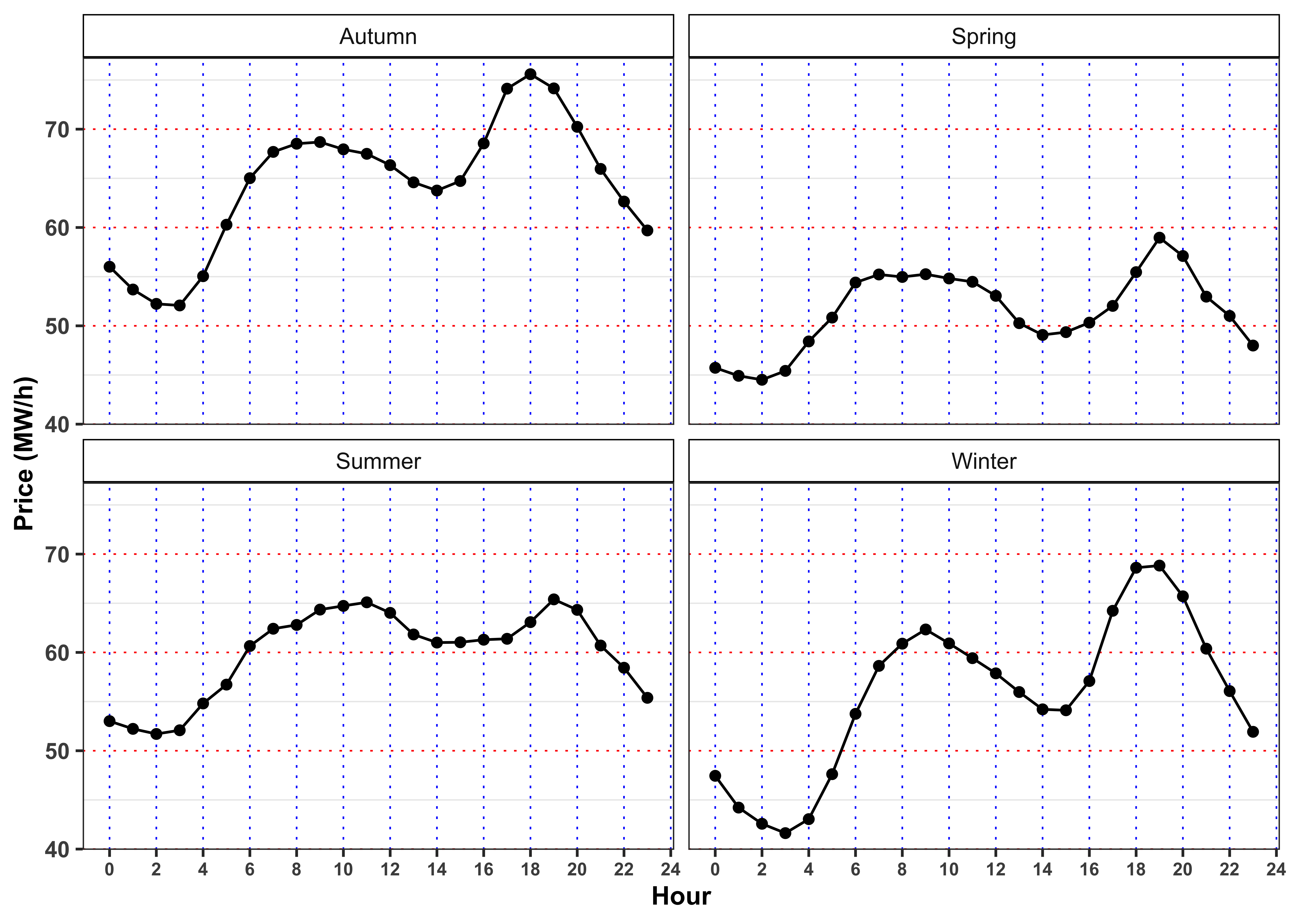
Grouping the dataset firstly by season and hour ($4\times 24$ groups) and then by month and hour ($12\times 24$ groups) compute:

1. Average electricity price
2. Average ratio between total production and total demand, i.e. prod/demand.

For both groups, answer to the following questions.

What is the meaning of a ratio between total production and total demand greater than 1? And greater than 1? Following the demand and supply law, what is the expected behavior of the price in such situations? Comment the results (max 200 words).

When the price reaches it’s minimum value? In such situation, does the ratio reach its maximum value? What happen when the prices reaches it’s maximum? Comment the results (max 200 words).

Insert the password to see the solution of Task Task-A5

Solution A.5

The minimum price for electricity by season and hour is reached, in mean, at 3:00 in all the seasons. Moreover, for all the seasons the ratio between production and demand is above 100% between 00:00 and 3:00 denoting a general excess of production with respect to the demand. Interestingly, when this ratio goes again above 100% again between 14:00 to 16:00 (except is summer) the price, in mean, reaches a relative minimum for the day.

On contrary the maximum price for the electricity, by season and hour is reached, in mean, at 19:00 except for Autumn (18:00). As expected, in the same period the production ratio reaches a minimum that for all the seasons is also a global minimum for the day.

In the monthly plots is highlighted the fact that is the drop in electricity price in 14:00 to 16:00 and the subsequent increase during the afternoon is smoothed going from May up to September.

Ratio (months)

Download

data %>%
  mutate(Month = lubridate::month(date_day, label = TRUE)) %>%
  mutate(prod = prod/demand) %>%
  group_by(Month, Hour) %>%
  summarise(prod = mean(prod, na.rm = TRUE)) %>%
  ggplot()+
  geom_line(aes(Hour, prod), color = "black")+
  geom_line(aes(Hour, 1), color = "red", linetype = "dashed")+
  facet_wrap(~Month)+
  theme_bw()+
  custom_theme+
  scale_y_continuous(breaks = seq(0, 1, 0.1), 
                     labels = paste0(seq(0, 1, 0.1)*100, " %"))+
  labs(color = NULL, y = "Production/Demand")

Figure 3: Mean Production/Demand by Month and Hour.

Price (months)

Download

data %>%
  mutate(Month = lubridate::month(date_day, label = TRUE)) %>%
  group_by(Month, Hour) %>%
  summarise(price = mean(price, na.rm = TRUE)) %>%
  ggplot()+
  geom_line(aes(Hour, price), color = "black")+
  facet_wrap(~Month)+
  theme_bw()+
  custom_theme+
  scale_y_continuous(breaks = seq(0, 100, 5), 
                     labels = seq(0, 100, 5))+
  labs(color = NULL, y = "Price")

Figure 4: Mean electricity prices by Month and Hour.

Ratio (seasons)

Download

data %>%
  mutate(prod = prod/demand) %>%
  group_by(Season, Hour) %>%
  summarise(prod = mean(prod, na.rm = TRUE)) %>%
  ggplot()+
  geom_line(aes(Hour, prod), color = "black")+
  geom_line(aes(Hour, 1), color = "red", linetype = "dashed")+
  facet_wrap(~Season)+
  theme_bw()+
  custom_theme+
  scale_x_continuous(breaks = seq(0, 24, 2))+
  scale_y_continuous(breaks = seq(0, 1, 0.1), 
                     labels = paste0(seq(0, 1, 0.1)*100, " %"))+
  labs(color = NULL, y = "Production/Demand")

Figure 5: Mean Production/Demand by Season and Hour.

Price (seasons)

Download

data %>%
  group_by(Season, Hour) %>%
  summarise(price = mean(price, na.rm = TRUE)) %>%
  ggplot()+
  geom_line(aes(Hour, price))+
  geom_point(aes(Hour, price))+
  facet_wrap(~Season)+
  theme_bw()+
  custom_theme+
  scale_x_continuous(breaks = seq(0, 24, 2))+
  scale_y_continuous(breaks = seq(0, 100, 10))+
  labs(color = NULL, y = "Price (MW/h)")

Figure 6: Mean electricity prices by Season and Hour.

3.2 Problem B: Model hourly electricity price

3.2.1 Task B.1

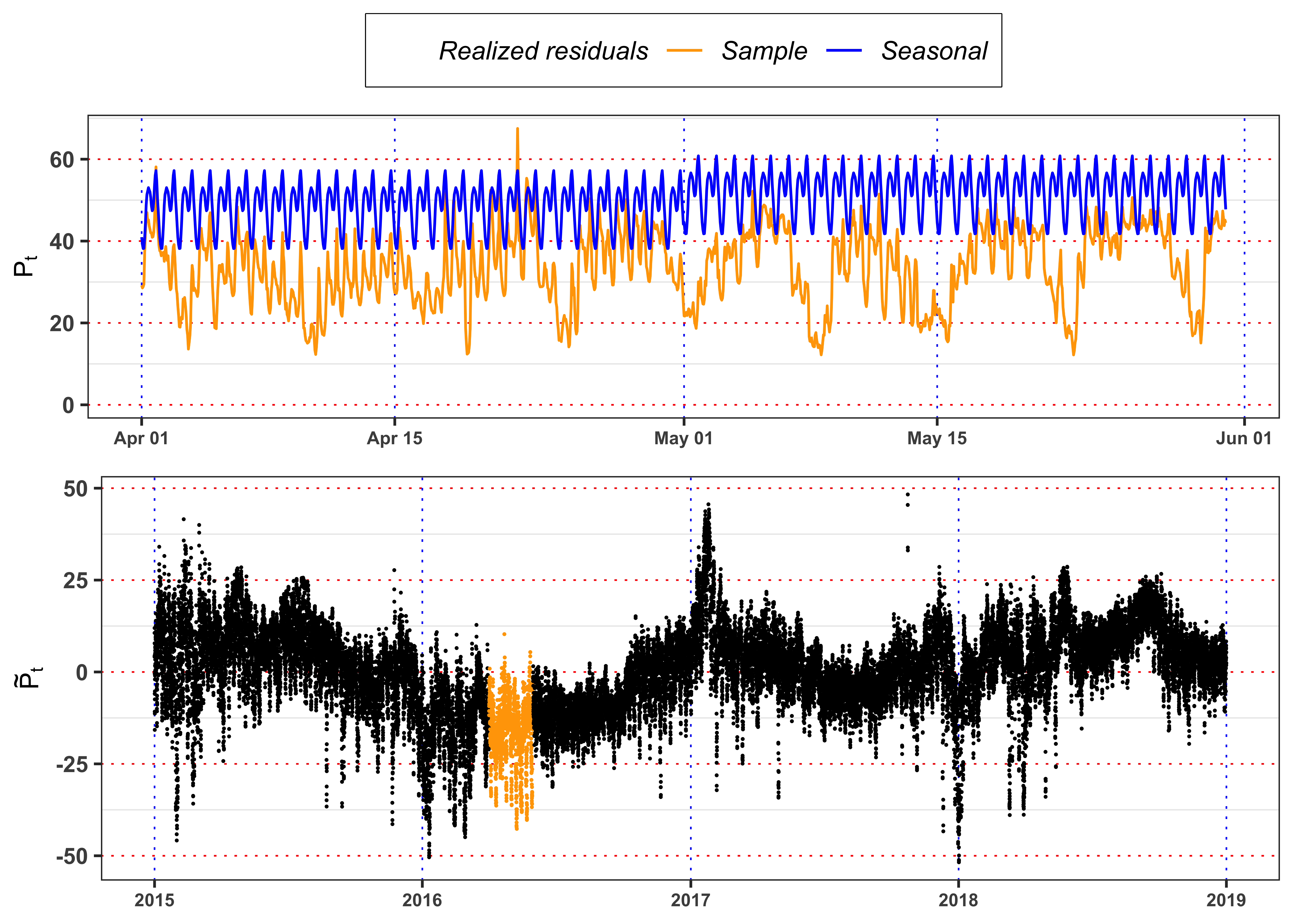
Let’s define and estimate a model for the hourly electricity price. First of all, we have to define a seasonal function to remove deterministic patterns during the year and the day. Hence, we take into account a function of the form: $$\begin{array}{r}{\overline{P}}_t=p_0+H(t)+M(t)\end{array}$$ where $H(t)$ stands for: $$H(t)=\{\begin{array}{l}{H}_1\text{Hour}=1\\ H_2\text{Hour}=2\\ ⋮\\ H_{23}\text{Hour}=23\end{array}$$ and $M(t)$ for: $$M(t)=\{\begin{array}{l}{M}_2\text{Month}=\text{February}\\ ⋮\\ M_{12}\text{Month}=\text{December}\end{array}$$ It follows that, by construction, $p_0$ captures the $\text{Hour}=0$ and $\text{Month}=\text{January}$. Estimate the parameters of the models using OLS. Then, compute the seasonal price ${\overline{P}}_t$ and the deseasonalized time series, i.e.  $${\tilde{P}}_t=P_t-{\overline{P}}_t$$ Plot ${\overline{P}}_t$ and ${\tilde{P}}_t$.

Insert the password to see the solution of Task Task-B1

Solution B.1

# Model dataset 
df_fit <- data
# Factor Variables
df_fit$Hour_ <- as.factor(df_fit$Hour)
df_fit$Month_ <- as.factor(df_fit$Month)
df_fit$Season_ <- as.factor(df_fit$Season)
# Seasonal model 
seasonal_model <- lm(price ~ Hour_ + Month_, data = df_fit) 
# Predicted seasonal mean 
df_fit$price_bar <- predict(seasonal_model, newdata = df_fit)
# Fitted residuals 
df_fit$price_tilde <- df_fit$price - df_fit$price_bar

seasonal_model %>%
  broom::glance() %>%
  knitr::kable()

Table 1: Seasonal model statistics for ${\overline{P}}_t$.

r.squared	adj.r.squared	sigma	statistic	p.value	df	logLik	AIC	BIC	deviance	df.residual	nobs
0.3178848	0.3172228	11.73688	480.1323	0	34	-136089.5	272251.1	272555.8	4825399	35029	35064

seasonal_model %>%
  broom::tidy() %>%
  knitr::kable()

Table 2: AR(1) estimates for ${\overline{P}}_t$.

term	estimate	std.error	statistic	p.value
(Intercept)	54.3007020	0.3696587	146.8941686	0.0000000
Hour_1	-1.7790349	0.4342528	-4.0967725	0.0000420
Hour_2	-2.7812936	0.4342528	-6.4047801	0.0000000
Hour_3	-2.7334839	0.4342528	-6.2946835	0.0000000
Hour_4	-0.2004517	0.4342528	-0.4616015	0.6443700
Hour_5	3.3283436	0.4342528	7.6645301	0.0000000
Hour_6	7.9087201	0.4342528	18.2122491	0.0000000
Hour_7	10.4300068	0.4342528	24.0182838	0.0000000
Hour_8	11.2295140	0.4342528	25.8593939	0.0000000
Hour_9	12.0915127	0.4342528	27.8444096	0.0000000
Hour_10	11.5433949	0.4342528	26.5822007	0.0000000
Hour_11	11.0641205	0.4342528	25.4785246	0.0000000
Hour_12	9.7660096	0.4342528	22.4892268	0.0000000
Hour_13	7.6069815	0.4342528	17.5174038	0.0000000
Hour_14	6.4553320	0.4342528	14.8653781	0.0000000
Hour_15	6.7521629	0.4342528	15.5489222	0.0000000
Hour_16	8.7482615	0.4342528	20.1455502	0.0000000
Hour_17	12.3532717	0.4342528	28.4471900	0.0000000
Hour_18	15.0938193	0.4342528	34.7581398	0.0000000
Hour_19	16.2539220	0.4342528	37.4296313	0.0000000
Hour_20	13.7690144	0.4342528	31.7073709	0.0000000
Hour_21	9.4329911	0.4342528	21.7223498	0.0000000
Hour_22	6.4771389	0.4342528	14.9155953	0.0000000
Hour_23	3.1923340	0.4342528	7.3513264	0.0000000
Month_2	-8.3290915	0.3115812	-26.7316899	0.0000000
Month_3	-13.7664987	0.3042645	-45.2451707	0.0000000
Month_4	-13.3461258	0.3067895	-43.5025441	0.0000000
Month_5	-9.7446337	0.3042645	-32.0268521	0.0000000
Month_6	-3.4205772	0.3067895	-11.1495884	0.0000000
Month_7	-1.2417608	0.3042645	-4.0811886	0.0000449
Month_8	-2.6181552	0.3042645	-8.6048663	0.0000000
Month_9	-0.7831501	0.3067895	-2.5527274	0.0106925
Month_10	1.8490054	0.3042645	6.0769674	0.0000000
Month_11	2.2175860	0.3067895	7.2283624	0.0000000
Month_12	3.7650571	0.3042645	12.3742904	0.0000000

Download

plot_seasonal <- df_fit %>%
  filter(Year == 2016 & Month %in% c(4:5) & Day %in% c(1:30))%>%
  ggplot()+
  geom_line(aes(date, price, color = "sample"))+
  geom_line(aes(date, price_bar, color = "seasonal"))+
  geom_line(aes(date, 0, color = "realized"), alpha = 0)+
  labs(x = NULL, y = TeX("$P_t$"), color = NULL)+
  scale_color_manual(values = c(sample = "orange", realized = "black", seasonal = "blue"),
                     labels = c(sample = "Sample", realized = "Realized residuals", seasonal = "Seasonal"))+
  theme_bw()+
  custom_theme
plot_eps <- df_fit %>%
  mutate(
    type = ifelse(Year == 2016 & Month %in% c(4:5) & Day %in% c(1:30), "col", "nocol") 
  ) %>%
  ggplot()+
  geom_point(aes(date, price_tilde, color = type), size = 0.05)+
  labs(x = NULL, y = TeX("$\\tilde{P}_t$"), color = NULL)+
  scale_color_manual(values = c(col = "orange", nocol = "black"))+
  theme_bw()+
  custom_theme+
  theme(legend.position = "none")

gridExtra::grid.arrange(plot_seasonal, plot_eps, ncol = 1)

Figure 7: Realized, seasonal and deseasonalized time series of electricity price in Spain. Years 2015-2018.

3.2.2 Task B.2

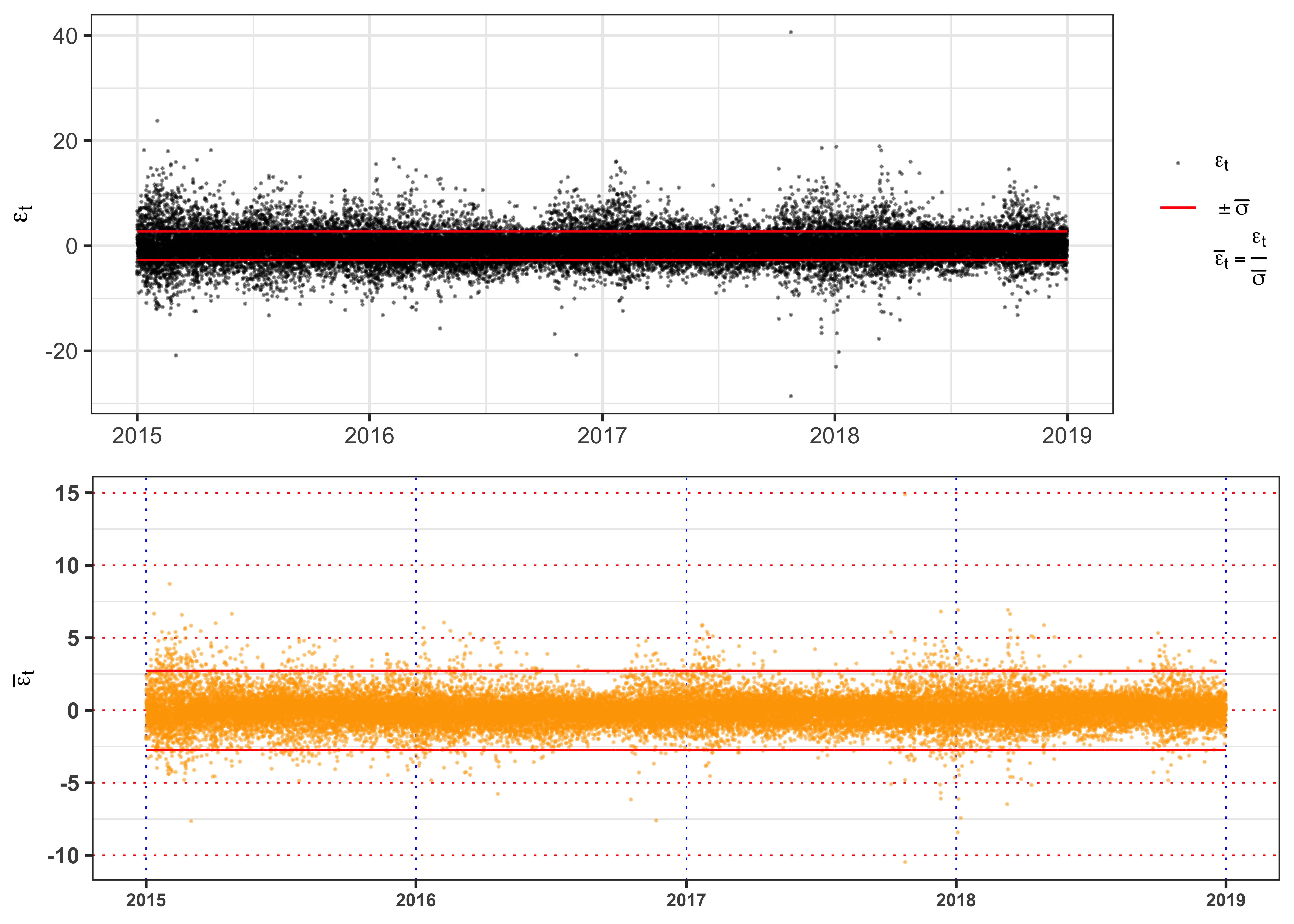
Estimate an autoregressive model (AR(1)) on the deseasonalized time series, i.e. $$\begin{array}{r}{\tilde{P}}_t=\varphi {\tilde{P}}_{t-1}+{\epsilon }_t\end{array}$$ Is the estimated model stationary? Comment and justify your answer.

Hint: in order to answer consider the stationarity condition on the parameters.

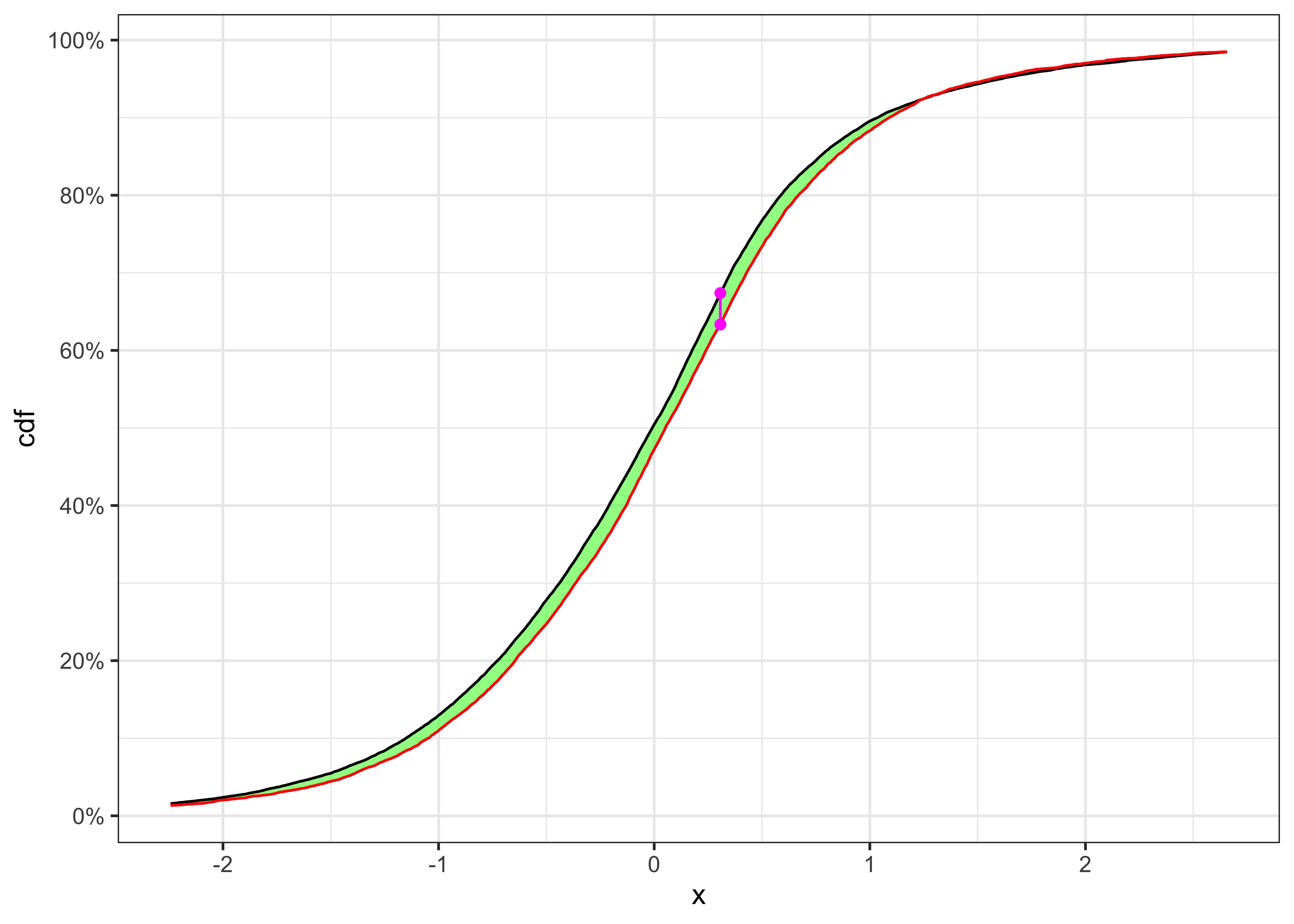
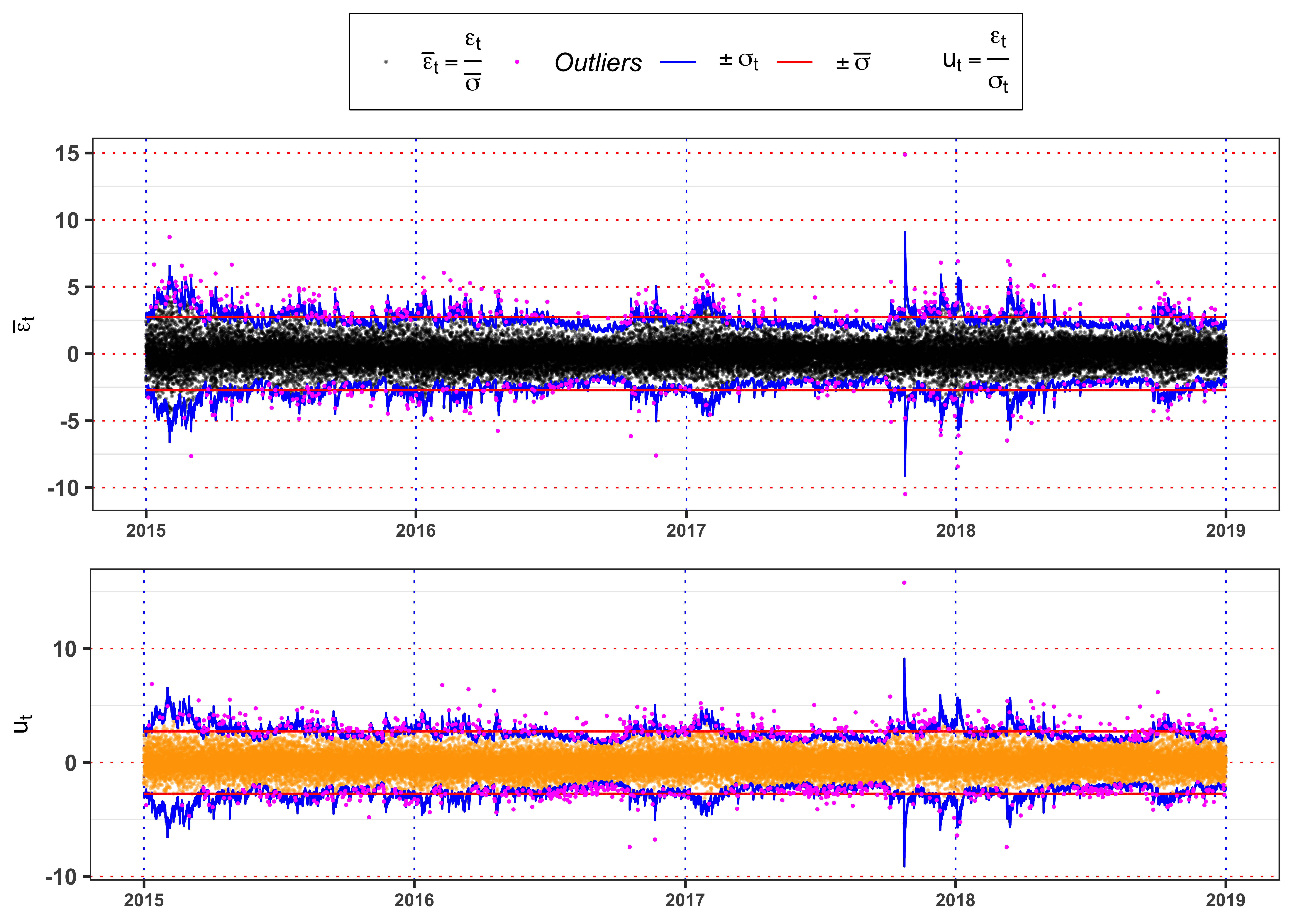
Then, compute the fitted residuals ${\epsilon }_t$ and their standard deviation as: $$\overline{\sigma }=\mathbb{S}d\{{\epsilon }_t\}=\sqrt{\frac{1}{n-1}\sum _{t=1}^n{\epsilon }_t^2}\text{,}$$ and the standardized residuals as $$\overline{{\epsilon }_t}=\frac{{\epsilon }_t}{\overline{\sigma }}\text{.}$$ Are $\overline{{\epsilon }_t}$ identically distributed? Answer with a formal statistics test with confidence level $\alpha =0.05$. (see for example see the two sample Kolmogorov-Smirnov test).

Insert the password to see the solution of Task Task-B2

Solution B.2

# AR model 
AR_model <- lm(price_tilde ~ I(lag(price_tilde, 1))-1, data = df_fit)
# Fitted values 
df_fit$price_tilde_hat <- predict(AR_model, newdata = df_fit)
# Fitted residuals 
df_fit$eps <- df_fit$price_tilde - df_fit$price_tilde_hat 
# Estimated constant standard deviation 
df_fit$sigma_bar <- sd(df_fit$eps, na.rm = TRUE)*sqrt(nrow(df_fit)/(nrow(df_fit)-1))
# Standardized residuals 
df_fit$std_eps <- df_fit$eps/df_fit$sigma_bar
df_fit <- df_fit[-1,]

Table 3: AR(1) statistics for ${\tilde{P}}_t$.

r.squared	adj.r.squared	sigma	logLik	AIC	BIC	deviance	df.residual	nobs
0.9458574	0.9458559	2.729713	-84961.89	169927.8	169944.7	261258.7	35062	35063

Table 4: AR(1) estimates for ${\tilde{P}}_t$.

term	estimate	std.error	statistic	p.value
$$\phi$$	0.9725531	0.0012427	782.6393	0

Since 0.973 is less than 1 in absolute value the AR(1) is stationary. However, it is still present volatility clustering that makes the residuals non-stationary. The ADF-test, where $H_0:\varphi =1$ (i.e. the process is non-stationary). If we reject $H_0$ the process is stationary, otherwise it is explosive, i.e. non-stationary.

Table 5: ADF-test on ${\tilde{P}}_t$.

statistic	p.value	parameter	method	lags	H0
-10.66521	0.01	20	Augmented Dickey-Fuller Test	20	Rejected (stationary)

Download

plot_eps <- ggplot(df_fit)+
  geom_point(aes(date, eps, color = "eps"), size = 0.1, alpha = 0.4)+
  geom_line(aes(date, sigma_bar, color = "sigma"), size = 0.4)+
  geom_line(aes(date, -sigma_bar, color = "sigma"), size = 0.4)+
  geom_line(aes(date, 0, color = "std_eps"), alpha = 0)+
  labs(x = NULL, y = TeX("$\\epsilon_t$"), color = NULL)+
  custom_theme+
  scale_color_manual(values = c(eps = "black", sigma = "red", std_eps = "darkorange"),
                     labels = c(eps = TeX("$\\epsilon_t$"), 
                                sigma = TeX("$\\pm\\bar{\\sigma}$"), 
                                std_eps = TeX("$\\bar{\\epsilon}_t = \\frac{\\epsilon_t}{\\bar{\\sigma}}$")))+
  theme_bw()
plot_std_eps <- ggplot(df_fit)+
  geom_point(aes(date, std_eps), color = "orange", size = 0.1, alpha = 0.4)+
  geom_line(aes(date, sigma_bar), color = "red", size = 0.4)+
  geom_line(aes(date, -sigma_bar), color = "red", size = 0.4)+
  labs(x = NULL, y = TeX("$\\bar{\\epsilon}_t$"), color = NULL)+
  theme_bw()+
  custom_theme+
  theme(legend.position = "none")

gridExtra::grid.arrange(plot_eps, plot_std_eps)

Figure 8: AR(1) residuals and standardized residuals with $\pm$ one standard deviation for the deasonalized electricity price in Spain. Years 2015-2018.

The graph above shows clearly that the standardized residuals presents volatility clusters, hence the time series of ${\overline{ϵ}}_t$ will be not identically distributed. A formal way to test it, is a two sample Kolmogorov-Smirnov.

Download

solarr::ks_test_ts(na.omit(df_fit$std_eps), ci = 0.01, seed = 1, plot = TRUE)

Figure 9: Two samples cdfs and KS-statistic (magenta) for ${\overline{ϵ}}_t$.

kab <- solarr::ks_test_ts(na.omit(df_fit$std_eps), ci = 0.01, seed = 1) %>%
  mutate_if(is.numeric, format, digits = 4, scientific = FALSE)
colnames(kab) <- c("$$\\textbf{Index split}$$", "$$\\alpha$$", "$$n_1$$", "$$n_2$$", 
                   "$$KS_{n_1, n_2}$$", "$$\\textbf{Critical Level}$$", "$$H_0$$")
knitr::kable(kab, booktabs = TRUE, escape = FALSE, align = 'c')%>%
  kableExtra::row_spec(0, color = "white", background = "green") 

Table 6: KS test for ${\overline{ϵ}}_t$.

$$\mathbf{\text{Index split}}$$	$$\alpha$$	$$n_1$$	$$n_2$$	$$K{S}_{n_1,n_2}$$	$$\mathbf{\text{Critical Level}}$$	$$H_0$$	NA
24388	1%	24388	10675	0.04047	0.00004769	0.01889	Rejected

The null hypothesis of independence and identically distribution is rejected, hence we have to define a model for the conditional variance of the process.

3.2.3 Task B.3

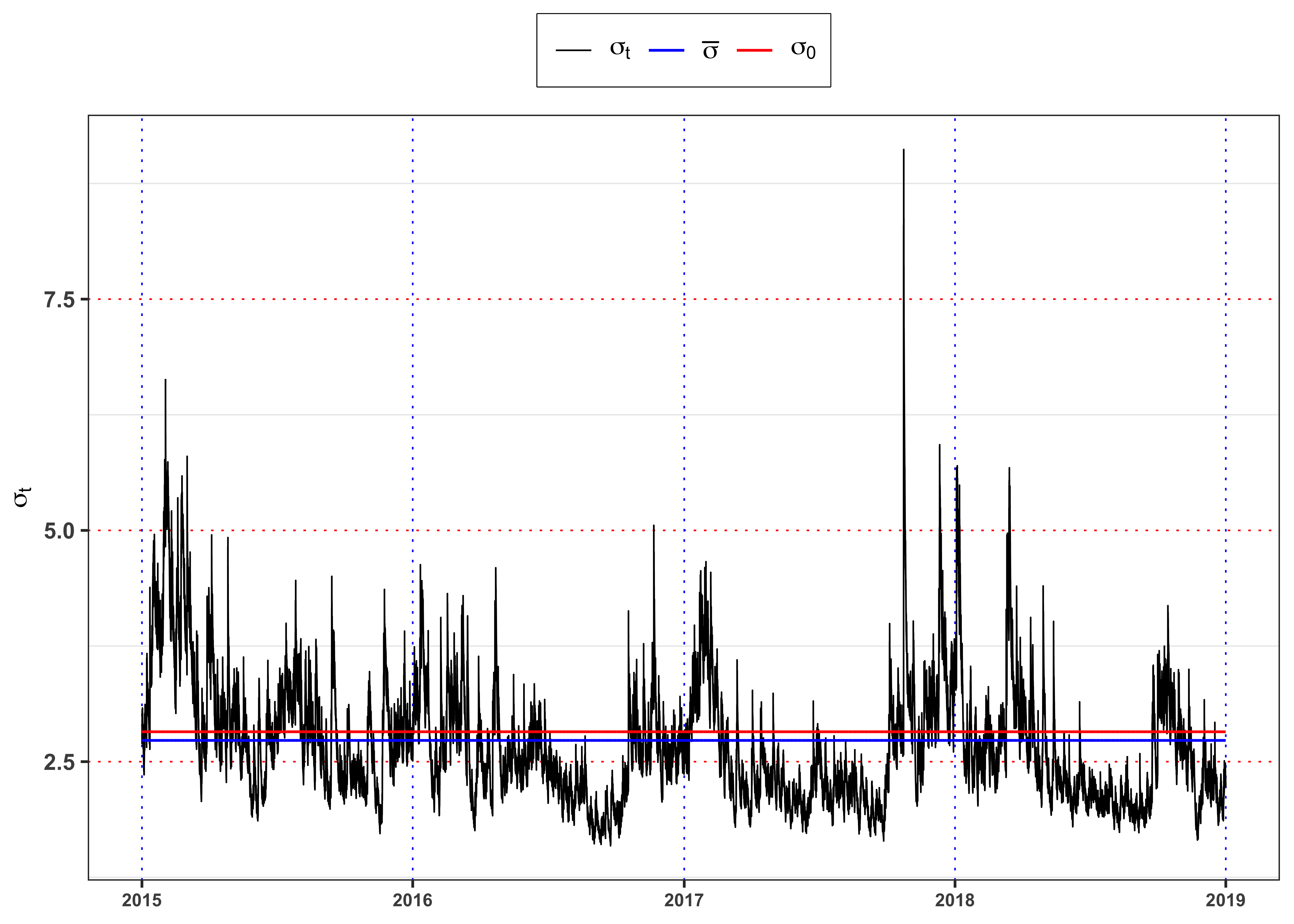
A model for the conditional variance is the GARCH(p,q) model. Let’s consider a GARCH(1,2) model under the normality assumption., i.e.  $$\begin{array}{rl}& {\epsilon }_t={\sigma }_t{u}_t\\ & {\sigma }_t^2=\omega +{\alpha }_1{\epsilon }_{t-1}^2+{\beta }_1{\sigma }_{t-1}^2+{\beta }_2{\sigma }_{t-2}^2\\ & u_t\sim \mathcal{N}(0,1)\end{array}$$

Is the estimated model stationary? Hint: in order to answer consider the stationarity condition on the parameters.

Compute the long-term variance under the GARCH(1,1) model, i.e. $\mathbb{E}\{{\sigma }_t^2\}$, and compare it with the variance estimated in Task B.2 (i.e. ${\overline{\sigma }}^2$). Are the two variances similar? Comment the results.

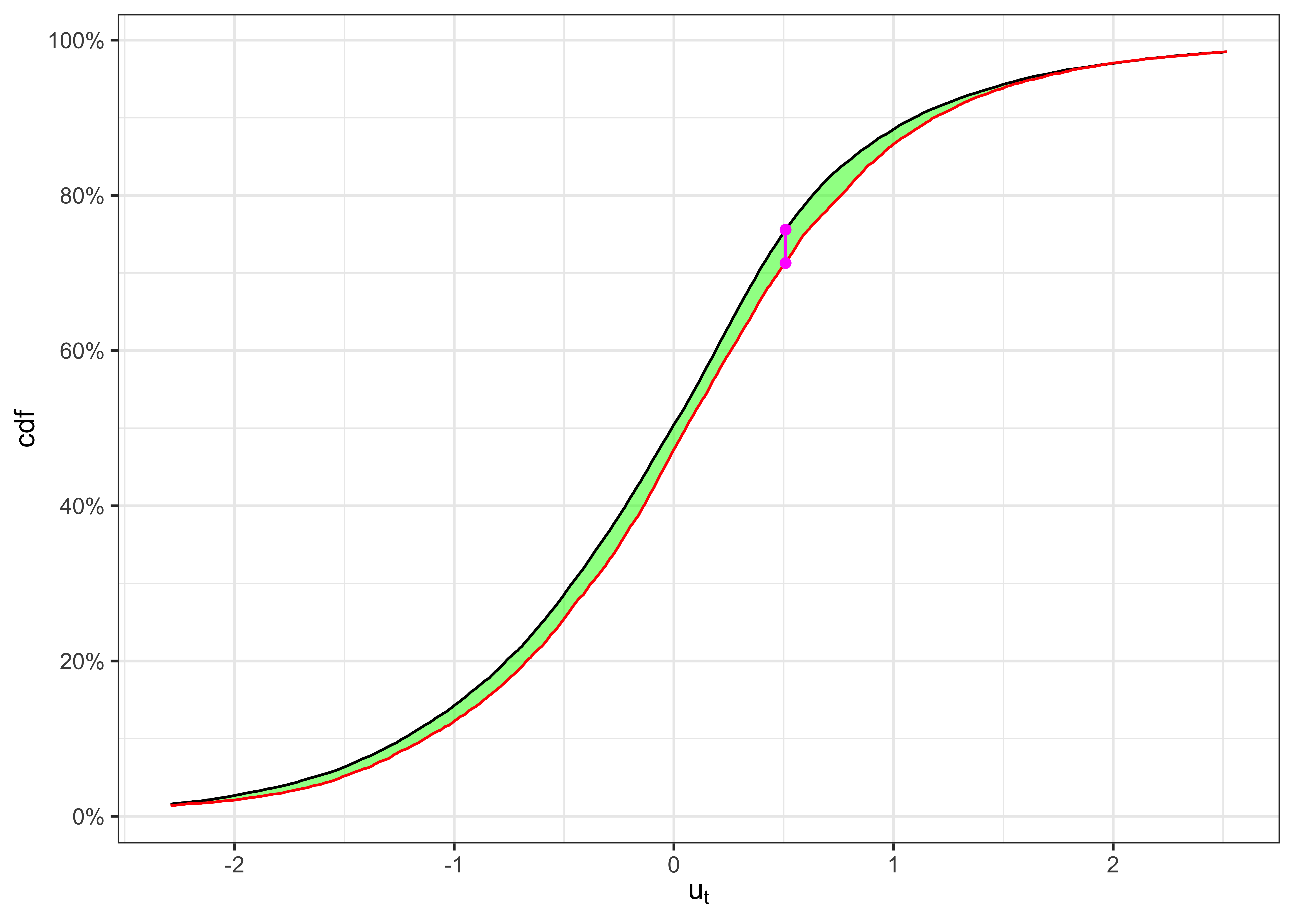
Define the standardized GARCH residuals as: $$u_t=\frac{{\epsilon }_t}{{\sigma }_t}$$ Are now the standardized residuals identically distributed? Answer using the same test used in Task B.2. Is the normality assumption satisfied on the fitted residuals? Answer with a formal test and a $\alpha =0.01$.

Hint: see for example see the Kolmogorov-Smirnov test.

Insert the password to see the solution of Task Task-B3

Solution B.3

# Variance specification
GARCH_spec <- rugarch::ugarchspec(
  variance.model = list(model = "sGARCH", garchOrder = c(1,2), external.regressors = NULL),
  mean.model = list(armaOrder = c(0,0), include.mean = FALSE), distribution.model = "norm")
# GARCH fitted model
GARCH_model <- rugarch::ugarchfit(data = df_fit$eps, spec = GARCH_spec, out.sample = 0)
# Fitted standard deviation
df_fit$sigma <- GARCH_model@fit$sigma
# Long-term standard deviation
df_fit$sigma_0 <- sqrt(GARCH_model@fit$coef[1]/(1-sum(GARCH_model@fit$coef[-1])))
# Fitted residuals
df_fit$ut <- df_fit$eps/df_fit$sigma

kab <- tibble(
  params = c("$$\\omega$$", "$$\\alpha_1$$", "$$\\beta_1$$", "$$\\beta_2$$"),
  estimates = GARCH_model@fit$coef,
  se.coef = GARCH_model@fit$se.coef
) %>%
  mutate_if(is.numeric, format, digits = 3, scientific = FALSE) 
knitr::kable(kab, booktabs = TRUE, escape = FALSE, align = 'c') %>%
  kableExtra::row_spec(0, color = "white", background = "green") 

Table 7: GARCH(1,2) estimates for $u_t$.

params	estimates	se.coef
$$\omega$$	0.0407	0.0043340
$${\alpha }_1$$	0.0378	0.0008108
$${\beta }_1$$	0.2161	0.0000111
$${\beta }_2$$	0.7409	0.0000111

Since the sum ${\alpha }_1+{\beta }_1+{\beta }_2=$ 0.995 is less than 1 in absolute value the model is stationary.

Download

plot_std_eps <- ggplot(df_fit)+
  geom_point(aes(date, std_eps, color = "eps"), size = 0.1, alpha = 0.4)+
  geom_line(aes(date, sigma, color = "sigma"), size = 0.4)+
  geom_line(aes(date, -sigma, color = "sigma"), size = 0.4)+
  geom_line(aes(date, sigma_bar, color = "sigma_bar"), size = 0.4)+
  geom_line(aes(date, -sigma_bar, color = "sigma_bar"), size = 0.4)+
  geom_line(aes(date, 0, color = "std_eps"), alpha = 0)+
  geom_point(data = filter(df_fit, std_eps > sigma | std_eps < -sigma),
             aes(date, std_eps, color = "outliers"), size = 0.1)+
  labs(x = NULL, y = TeX("$\\bar{\\epsilon}_t$"), color = NULL)+
  scale_color_manual(values = c(eps = "black", outliers = "magenta",
                                sigma = "blue", sigma_bar = "red", std_eps = "darkorange"),
                     labels = c(eps = TeX("$\\bar{\\epsilon}_t = \\frac{\\epsilon_t}{\\bar{\\sigma}}$"), 
                                sigma_bar = TeX("$\\pm\\bar{\\sigma}$"), 
                                sigma = TeX("$\\pm\\sigma_t$"),
                                outliers = "Outliers",
                                std_eps = TeX("$u_t = \\frac{\\epsilon_t}{\\sigma_t}$")))+
  theme_bw()+
  custom_theme

plot_ut <- ggplot(df_fit)+
  geom_point(aes(date, ut), color = "orange", size = 0.1, alpha = 0.4)+
  geom_line(aes(date, sigma), color = "blue", size = 0.4)+
  geom_line(aes(date, -sigma), color = "blue", size = 0.4)+
  geom_line(aes(date, sigma_bar), color = "red", size = 0.4)+
  geom_line(aes(date, -sigma_bar), color = "red", size = 0.4)+
  geom_point(data = filter(df_fit, ut > sigma | ut < -sigma),
             aes(date, ut), color = "magenta", size = 0.1)+
  labs(x = NULL, y = TeX("$u_t$"), color = NULL)+
  theme_bw()+
  custom_theme+
  theme(legend.position = "none")

gridExtra::grid.arrange(plot_std_eps, plot_ut, heights = c(0.6, 0.4))

Figure 10: Standardized residuals and GARCH standardized residuals with $\pm$ one GARCH standard deviation. Years 2015-2018.

Download

solarr::ks_test_ts(na.omit(df_fit$ut), ci = 0.01, seed = 1, plot = TRUE) +
  labs(x = TeX("$u_t$"))

Figure 11: Two samples cdfs and KS-statistic (magenta) for a $u_t$.

kab <- solarr::ks_test_ts(na.omit(df_fit$ut), ci = 0.01, seed = 1) %>%
  mutate_if(is.numeric, format, digits = 4, scientific = FALSE)
colnames(kab) <- c("$$\\textbf{Index split}$$", "$$\\alpha$$", "$$n_1$$", "$$n_2$$", 
                   "$$KS_{n_1, n_2}$$", "$$\\textbf{Critical Level}$$", "$$H_0$$")
knitr::kable(kab, booktabs = TRUE, escape = FALSE, align = 'c') %>%
  kableExtra::row_spec(0, color = "white", background = "green") 

Table 8: KS test for $u_t$.

$$\mathbf{\text{Index split}}$$	$$\alpha$$	$$n_1$$	$$n_2$$	$$K{S}_{n_1,n_2}$$	$$\mathbf{\text{Critical Level}}$$	$$H_0$$	NA
24388	1%	24388	10675	0.04295	0.00001238	0.01889	Rejected

Download

ggplot(df_fit)+
  geom_line(aes(date, sigma, color = "sigma"), size = 0.3)+
  geom_line(aes(date, sigma_0, color = "sigma0"))+
  geom_line(aes(date, sigma_bar, color = "sigma_bar"))+
  geom_line(aes(date, 0, color = "std_eps"), alpha = 0)+
  labs(x = NULL, y = TeX("$\\sigma_t$"), color = NULL)+
  scale_y_continuous(limits = c(min(df_fit$sigma), max(df_fit$sigma)))+
  scale_color_manual(values = c(sigma = "black", sigma0 = "red", sigma_bar = "blue"),
                     labels = c(sigma = TeX("$\\sigma_t$"), 
                                sigma0 = TeX("$\\sigma_0$"), 
                                sigma_bar = TeX("$\\bar{\\sigma}$")))+
  theme_bw()+
  custom_theme

Figure 12: GARCH(1,2) standard deviation ${\sigma }_t$ with long term mean ${\sigma }_0$ and standard deviation of the AR(1) residuals $\overline{\sigma }$.

3.2.4 Task B.4

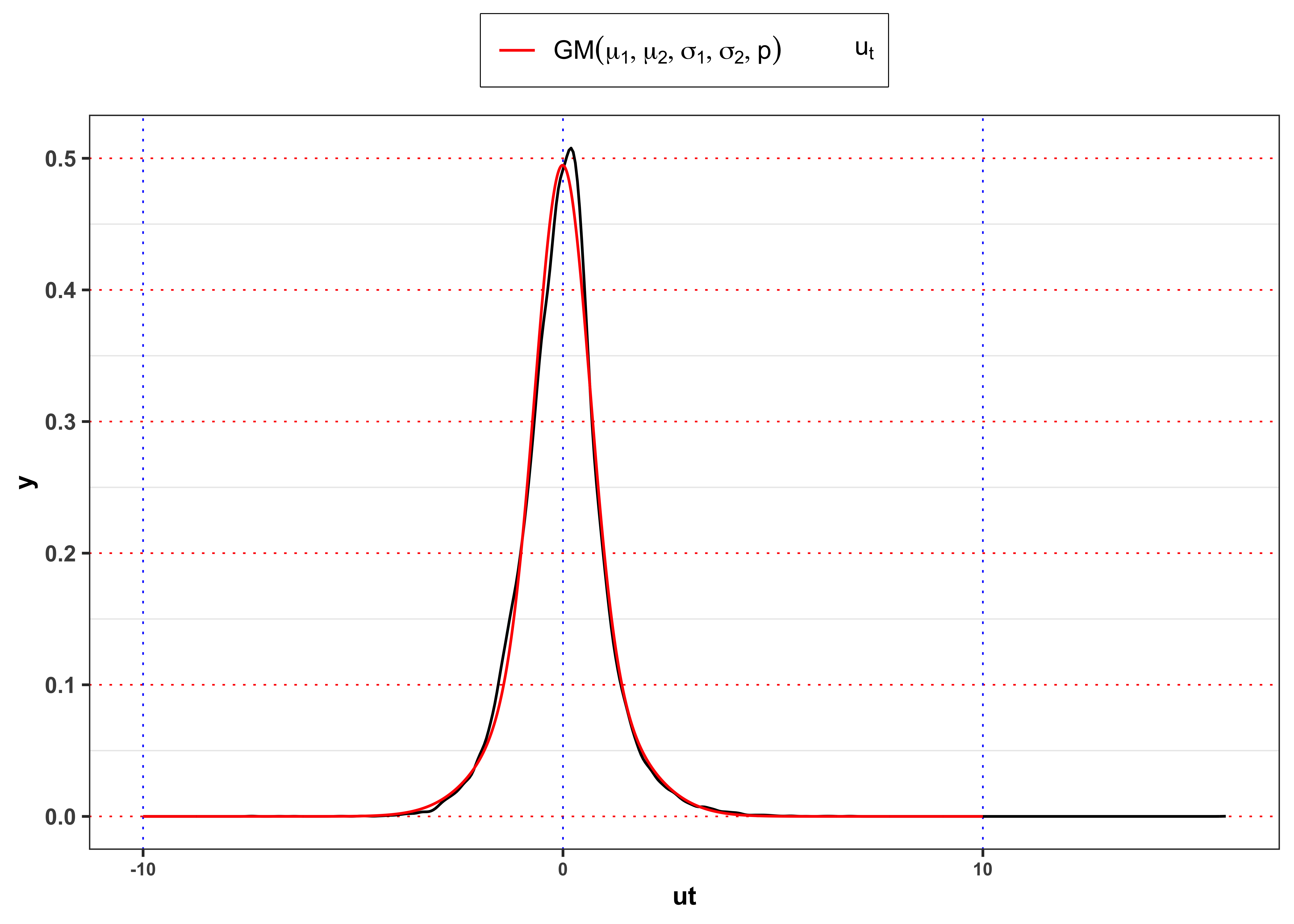
Let’s consider a Gaussian mixture model for the GARCH residuals, i.e.  $$u_t\sim B\cdot ({\mu }_1+{\sigma }_1{Z}_1)+(1-B)\cdot ({\mu }_2+{\sigma }_2{Z}_2)$$

where $B\sim \text{Bernoulli}(p)$, while $Z_1$ and $Z_2$ are standard normal. All are assumed to be independent. Estimate the parameters ${\mu }_1$, ${\mu }_2$, ${\sigma }_1$, ${\sigma }_2$ and $p$ with maximum likelihood (see here for an example). Consider the estimated parameters and give a possible interpretation of the two states, i.e. B = 1, B = 0.

Insert the password to see the solution of Task Task-B4

Solution B.4

grid <- seq(-10, 10, 0.01)
# Mixture model 
NM_model <- mclust::Mclust(df_fit$ut, G = 2, verbose = FALSE)
# Extract the parameters 
params <- c(NM_model$parameters$mean, sqrt(NM_model$parameters$variance$scale), NM_model$parameters$pro[1])
names(params) <- c("$$\\mu_1$$", "$$\\mu_2$$", "$$\\sigma_1$$", "$$\\sigma_2$$", "$$p_1$$")
bind_rows(params) %>%
  bind_cols(p2 = 1 - params[5], log_lik = NM_model$loglik, mu_u = mean(df_fit$ut), sd_u = sd(df_fit$ut)) %>% 
  mutate_if(is.numeric, format, digits = 4, scientific = FALSE) %>%
  knitr::kable(
    escape = FALSE,
    col.names = c("$$\\mu_1$$", "$$\\mu_2$$", 
                  "$$\\sigma_1$$", "$$\\sigma_2$$", "$$p_1$$", "$$1-p_1$$", 
                  "log-lik", "$$\\mathbb{E}\\{u_t\\}$$", "$$\\mathbb{S}d\\{u_t\\}$$"))

Table 9: Yearly Gaussian Mixture parameters.

$${\mu }_1$$	$${\mu }_2$$	$${\sigma }_1$$	$${\sigma }_2$$	$$p_1$$	$$1-p_1$$	log-lik	$$\mathbb{E}\{u_t\}$$	$$\mathbb{S}d\{u_t\}$$
-0.0113	0.01044	0.6337	1.385	0.6053	0.3947	-48467	-0.002722	1

Download

ggplot()+
  geom_density(data = df_fit, aes(ut), color = "black")+
  geom_line(aes(grid, 0, color = "ut"), alpha = 0)+
  geom_line(aes(grid, solarr::dmixnorm(grid, params[1:2], params[3:4], c(params[5], 1-params[5])), color = "nm"))+
  scale_color_manual(values = c(ut = "black", nm = "red"), 
                     labels = c(ut = TeX("$u_t$"), nm = TeX("$GM(\\mu_1, \\mu_2, \\sigma_1, \\sigma_2, p)$")))+
  theme_bw()+
  custom_theme+
  labs(color = NULL)

Figure 13: Yearly Gaussian Mixture vs Empirical densities.

Download

pdf <- solarr::dmixnorm(grid, params[1:2], params[3:4], c(params[5], 1-params[5]))
df_grid <- tibble(Month = lubridate::month(1, label = TRUE), grid = grid, pdf = pdf)
for(i in 2:12){
  df_grid <- bind_rows(df_grid, mutate(df_grid, Month = lubridate::month(i, label = TRUE)))
}
df_fit %>%
  mutate(Month = lubridate::month(date, label = TRUE)) %>%
  ggplot()+
  geom_density(aes(ut), color = "red")+
  geom_line(data = df_grid, aes(grid, pdf), color = "blue")+
  facet_wrap(~Month)+
  scale_x_continuous(limits = c(-5, 5))+
  theme_bw()+
  custom_theme

Figure 14: Yearly Gaussian Mixture vs Empirical monthly densities.

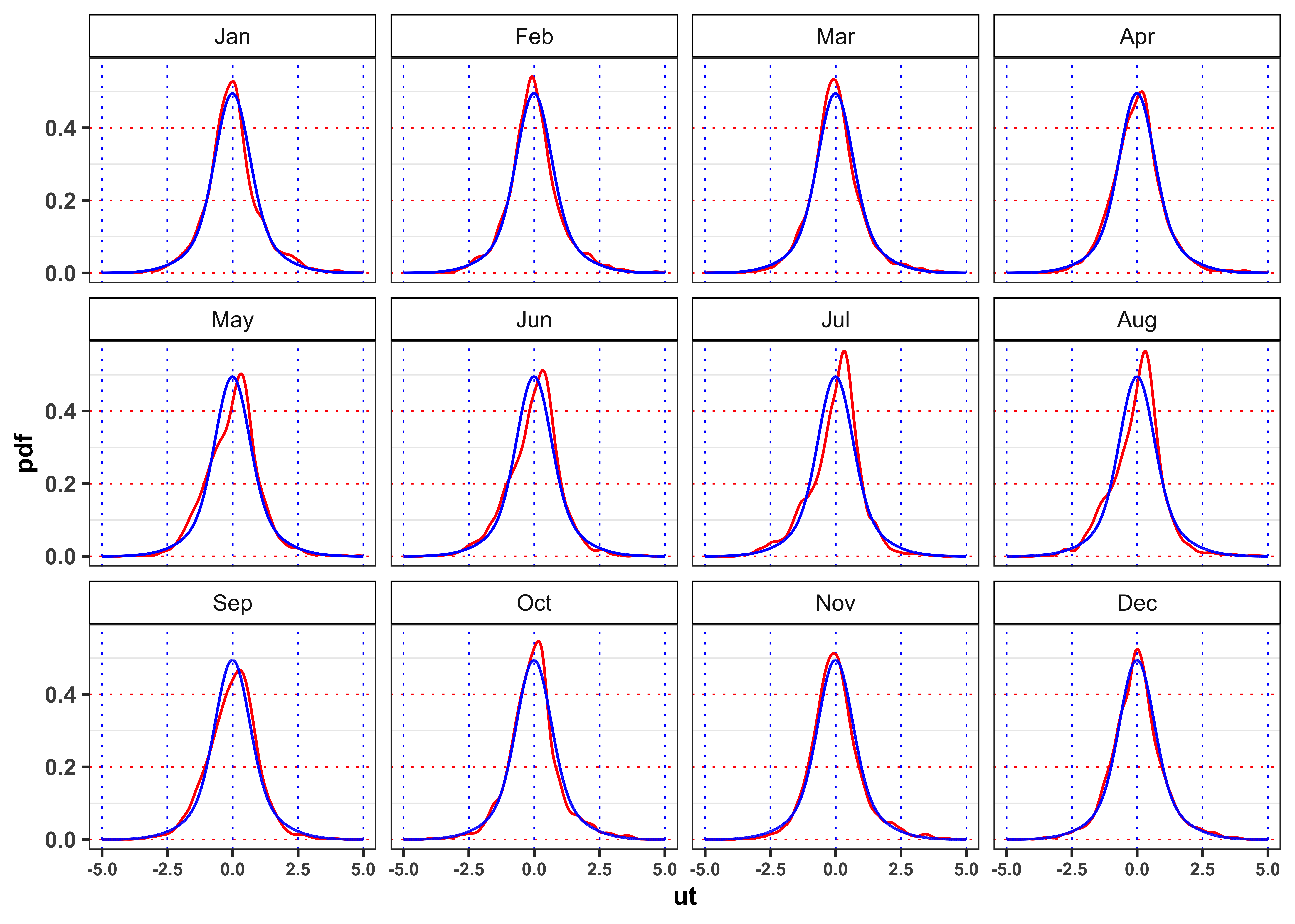
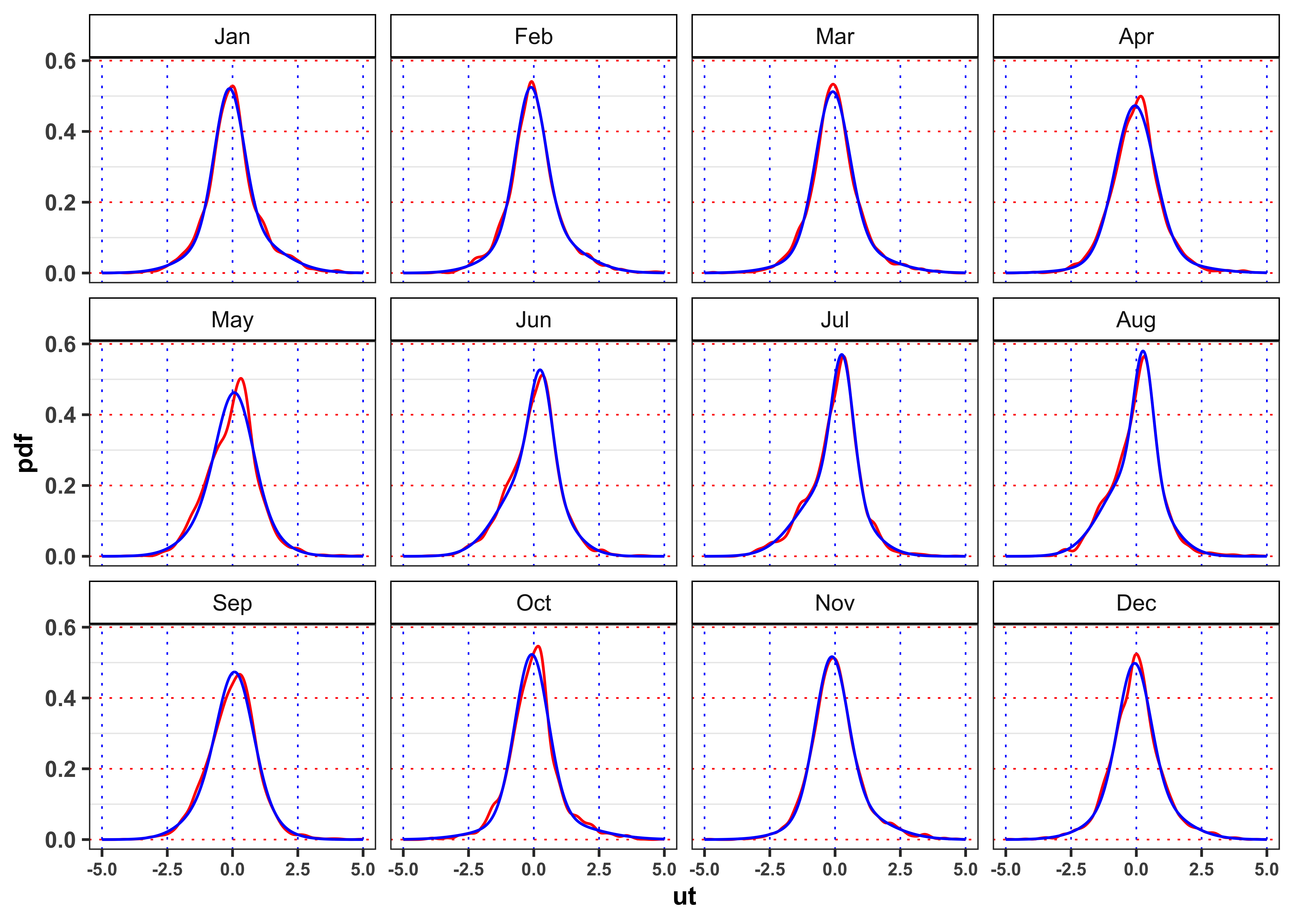
3.2.5 Task B.5

Let’s consider a monthly Gaussian mixture model for the GARCH residuals $u_{t,m}$, where the index $m=1,\dots ,12$ denotes the $m$-month, i.e. $$u_{t,m}\sim B_m\cdot Z_{m,1}+(1-B_m)\cdot Z_{m,2}$$ where all the random variables, i.e.  $$\begin{array}{rl}& B_m\sim \text{Bernoulli}(p_m)\\ & Z_{m,1}=\mathcal{N}({\mu }_{m,1},{\sigma }_{m,1}^2)\\ & Z_{m,2}=\mathcal{N}({\mu }_{m,2},{\sigma }_{m,2}^2)\end{array}$$ are assumed to be independent. Estimate the parameters for all the months with maximum likelihood.

Insert the password to see the solution of Task Task-B5

Solution B.5

date <- df_fit$date
x <- df_fit$ut
# Extract the month 
M <- lubridate::month(date)
# Initialize a dataset with all the variables 
data <- dplyr::tibble(Month = M, ut = x)
# Fitting monthly routine 
NM_mixture <- list()
for(i in 1:12){
  # Monthly data
  eps <- dplyr::filter(data, Month == i)$ut
  # Mixture model 
  NM_model <- mclust::Mclust(eps, G = 2, verbose = FALSE)
  # Extract the parameters 
  params <- c(NM_model$parameters$mean, sqrt(NM_model$parameters$variance$scale), NM_model$parameters$pro)
  names(params) <- c("mu1", "mu2", "sd1", "sd2", "p1", "p2")
  # Fitted parameters
  params <- dplyr::bind_rows(params)
  params$log_lik <- NM_model$loglik
  # Monthly data
  NM_mixture[[i]] <- dplyr::tibble(Month = i, params, nobs = length(eps))
}
NM_mixture <- dplyr::bind_rows(NM_mixture)

NM_mixture %>%
  mutate(Month = lubridate::month(Month, label = TRUE)) %>%
  mutate_if(is.numeric, format, digits = 2, scientific = FALSE) %>%
  knitr::kable(
    escape = FALSE,
    col.names = c("Month", "$$\\mu_1$$", "$$\\mu_2$$", 
                  "$$\\sigma_1$$", "$$\\sigma_2$$", "$$p_1$$", "$$1-p_1$$", 
                  "log-lik", "nobs"))

Table 10: Monthly Gaussian Mixture parameters.

Month	$${\mu }_1$$	$${\mu }_2$$	$${\sigma }_1$$	$${\sigma }_2$$	$$p_1$$	$$1-p_1$$	log-lik	nobs
Jan	-0.129	0.168	0.56	1.43	0.57	0.43	-4177	2976
Feb	-0.120	0.158	0.56	1.41	0.58	0.42	-3761	2712
Mar	-0.096	0.211	0.64	1.55	0.70	0.30	-4067	2976
Apr	-0.057	0.239	0.75	1.67	0.81	0.19	-3964	2880
May	0.089	-0.084	0.68	1.21	0.52	0.48	-4115	2976
Jun	-0.148	0.280	1.14	0.44	0.66	0.34	-3946	2880
Jul	-0.218	0.284	1.18	0.42	0.60	0.40	-4021	2976
Aug	-0.148	0.285	1.11	0.37	0.67	0.33	-3966	2976
Sep	-0.143	0.106	1.20	0.67	0.45	0.55	-3916	2880
Oct	-0.083	0.232	0.64	1.74	0.74	0.26	-4098	2976
Nov	-0.134	0.294	0.62	1.45	0.67	0.33	-3913	2880
Dec	-0.074	0.086	0.62	1.38	0.59	0.41	-4135	2975

Download

df_grid <- tibble()
for(i in 1:12){
  params <- unlist(NM_mixture[i,][2:7])
  pdf <- solarr::dmixnorm(grid, params[1:2], params[3:4], params[5:6])
  new_df <- tibble(Month = lubridate::month(i, label = TRUE), grid = grid, pdf = pdf)
  df_grid <- bind_rows(df_grid, new_df)
}
df_fit %>%
  mutate(Month = lubridate::month(date, label = TRUE)) %>%
  ggplot()+
  geom_density(aes(ut), color = "red")+
  geom_line(data = df_grid, aes(grid, pdf), color = "blue")+
  facet_wrap(~Month)+
  scale_x_continuous(limits = c(-5, 5))+
  theme_bw()+
  custom_theme

Figure 15: Yearly Gaussian Mixture vs monthly empirical densities.

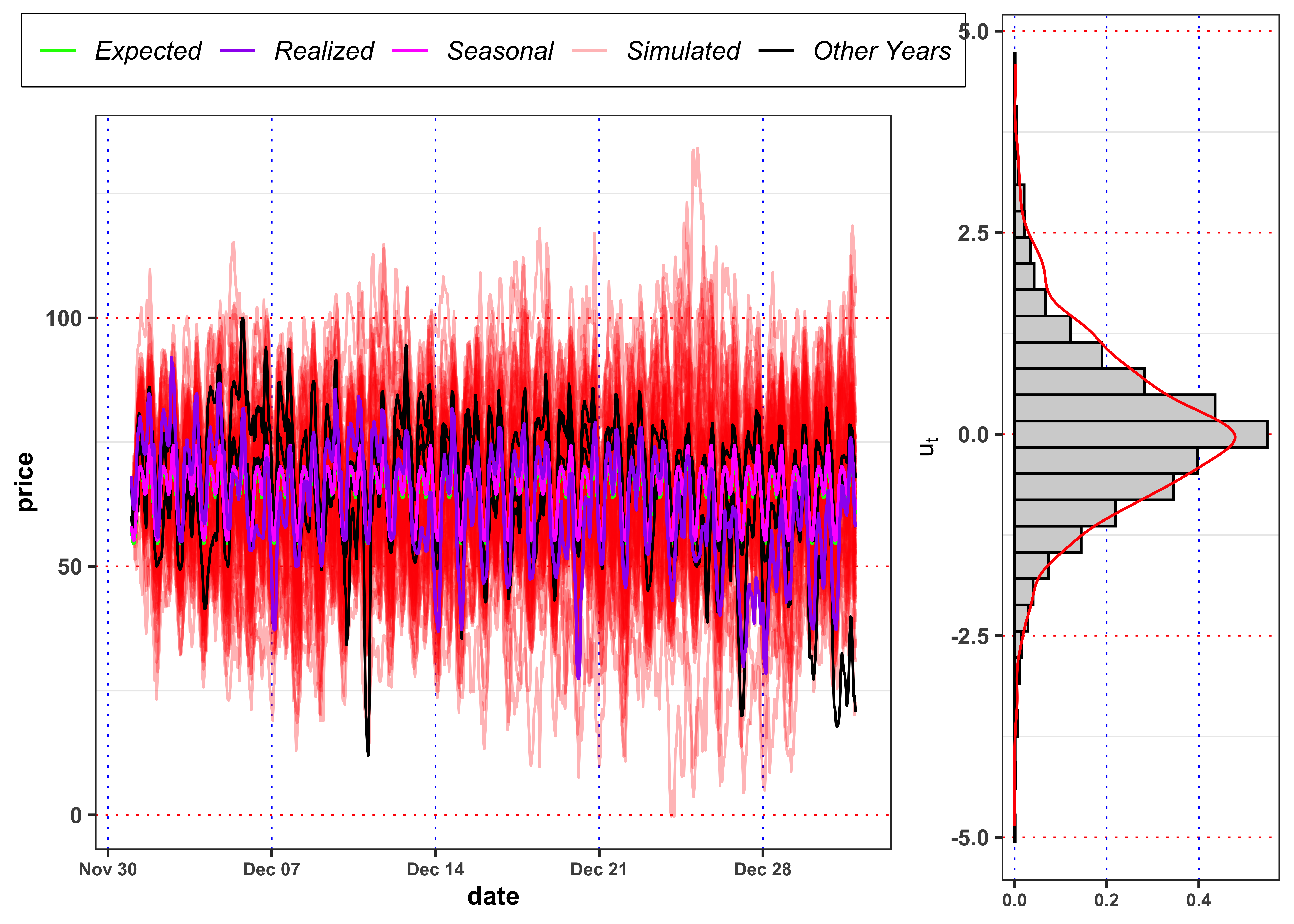
3.2.6 Task B.6

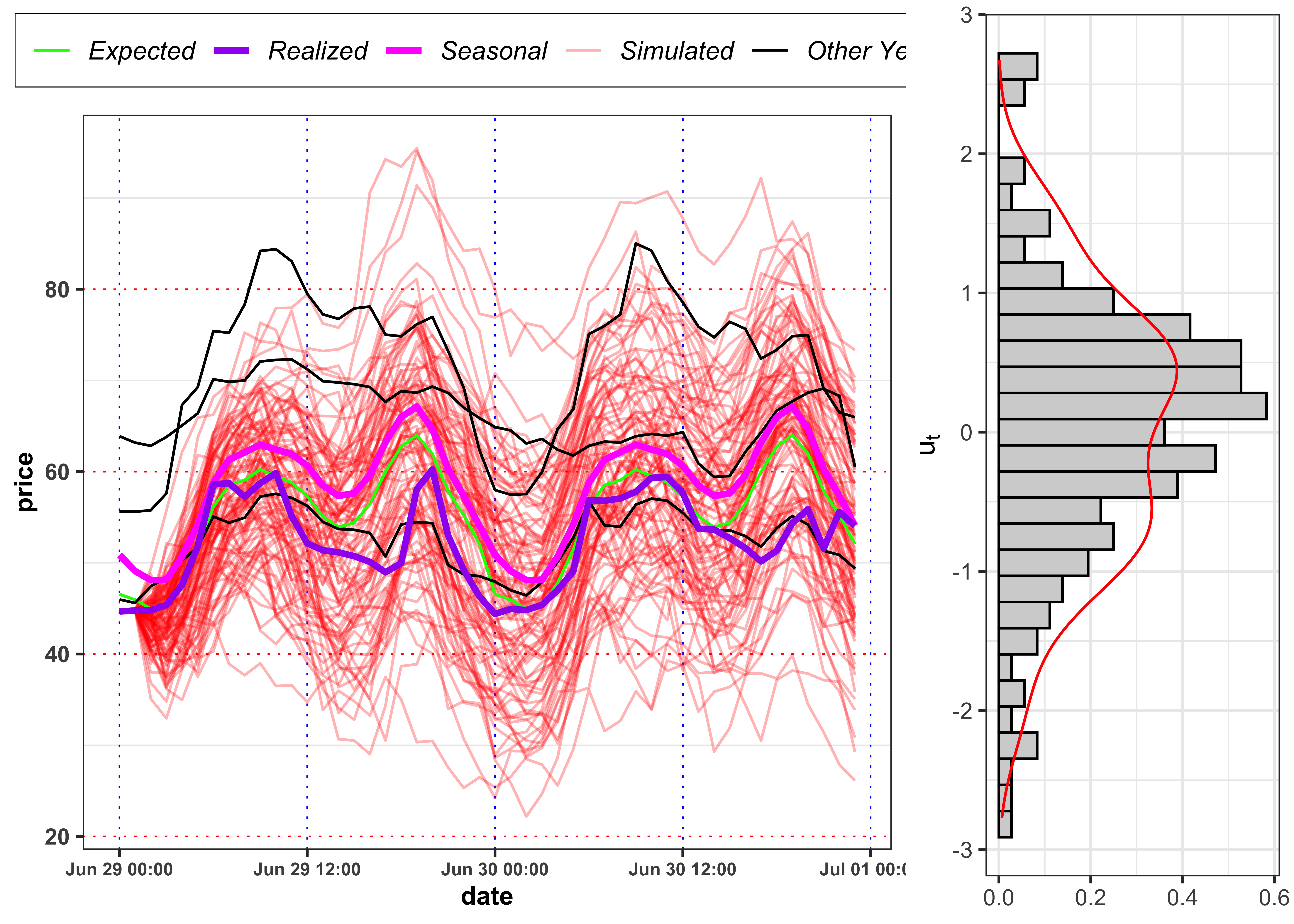
Let’s simulate hourly prices with the model and compare it with the empirical ones. You are free to choose between the basic Gaussian mixture and the monthly version. Then, consider the following two situations:

1. Projection A: You are 2017-06-28 (known) and you want to simulate 100 trajectories for the price from 2017-06-29 up to 2017-06-30 (1 day, 24 hours).

2. Projection B: You are in 2017-12-01 (known) and you want to simulate 100 trajectories for the price from 2017-12-02 up to 2017-12-31 (29 days, 696 hours).

Be careful in simulations to always set a seed for reproducibility.

• The distribution of the residuals in the Projection A are close to the empirical distribution of the residuals in that month? The situation in Projection B changes? Is the model able to forecast the short term movements of the electricity price? Comment the results.

Hint 1: For a graphical comparison between densities you can plot the empirical histograms of $u_t$ for the month $m=12$ (December) and the histograms of the simulated $u_t$ for the same month.

Hint 2: Think about the fact that the aim of our model is to try to reproduce the distribution of the electricity prices and not to forecast it’s short term movements (potential omitted values could improve the model performances).

Insert the password to see the solution of Task Task-B6

Solution B.6

Download

set.seed(1)
# Number of scenarios 
j_bar <- 100
day_date <- seq.Date(as.Date("2017-06-29"), as.Date("2017-06-30"), 1)

# Extract year, month and day
Y <- lubridate::year(day_date)[1]
M <- lubridate::month(day_date)[1]
D <- lubridate::day(day_date)

# Datasets 
df_emp <- filter(df_fit, Year == Y & Month == M & Day %in% D)
df_emp_plot <- filter(df_fit, Month == M & Day %in% D)
df_emp_plot <- right_join(select(df_emp, date, Month, Day, Hour), 
                          select(df_emp_plot, -date), by = c("Month", "Day", "Hour"))
# Simulated scenarios 
scenarios <- list()
for(j in 1:j_bar){
  # Initialize dataset 
  df_sim <- df_emp
  # Simulated standard normal 
  df_sim$ut <- rnorm(nrow(df_sim), mean = 0, sd = 1)
  df_sim$B <- 0
  # Single simulation
  for(i in 3:nrow(df_sim)){
    # Parameters 
    # Extract month 
    M_i <- lubridate::month(df_sim$date[i])
    # Gaussian mixture parameters
    NM <- unlist(NM_mixture[M_i, c(2:6)])
    # GARCH(1,1) parameters 
    GARCH <- GARCH_model@fit$coef
    # AR(1) parameters 
    phi <- AR_model$coefficients[1]
    # Simulation 
    # Simulated binomial 
    df_sim$B[i] <- rbinom(1, 1, prob = NM[5])
    # Simulated Gaussian mixture 
    df_sim$ut[i] <- df_sim$B[i]*(NM[1] + NM[3]*df_sim$ut[i]) + (1-df_sim$B[i])*(NM[2] + NM[4]*df_sim$ut[i])
    # Simulated GARCH std. deviation 
    df_sim$sigma[i] <- sqrt(GARCH[1] + GARCH[2]*df_sim$eps[i-1]^2 + GARCH[3]*df_sim$sigma[i-1]^2 + + GARCH[4]*df_sim$sigma[i-2]^2)
    # Simulated residuals 
    df_sim$eps[i] <- df_sim$sigma[i]*df_sim$ut[i]
    # Simulated deseasonalized price 
    df_sim$price_tilde[i] <- phi*df_sim$price_tilde[i-1] + df_sim$eps[i]
    # Seasonal mean 
    # H <- as.factor(lubridate::hour(df_sim$date[i])))
    # S <- as.factor(solarr::detect_season(df_sim$date[i]))
    # df_sim$price_bar[i] <- predict(seasonal_model, newdata = tibble(Hour_ = H, Season_ = S))
    # Simulated price 
    df_sim$price[i] <- df_sim$price_tilde[i] + df_sim$price_bar[i]
  }
  scenarios[[j]] <- dplyr::bind_cols(j = j, df_sim)
}

df_scenarios <- bind_rows(scenarios) %>%
  group_by(Hour) %>%
  mutate(e_price = mean(price))

plt_sim <-ggplot()+
  geom_line(data = df_scenarios, aes(date, price, group = j, color = "sim"), alpha = 0.3)+
  geom_line(data = df_scenarios, aes(date, e_price, group = j, color = "expected"))+
  geom_line(data = df_emp_plot, aes(date, price, group = Year, color = "year"))+
  geom_line(data = df_emp_plot, aes(date, price_bar, group = Year, color = "seasonal"), size = 1.2)+
  geom_line(data = df_emp, aes(date, price, color = "realized"), size = 1.2)+
  scale_color_manual(values = c(sim = "red", seasonal = "magenta", expected = "green", 
                                realized = "purple", year = "black"), 
                     labels = c(sim = "Simulated", seasonal = "Seasonal", 
                                expected = "Expected", 
                                realized = "Realized", year = "Other Years"))+
  theme_bw()+
  custom_theme+
  labs(color = NULL)

plt_hist <- ggplot()+
  geom_histogram(data = df_emp_plot, aes(ut, after_stat(density)),
                 color = "black", fill = "lightgray")+
  geom_density(data = df_sim, aes(ut), color = "red")+
  theme_bw()+
  labs(x = TeX("$u_t$"), y = NULL)+
  coord_flip()

gridExtra::grid.arrange(plt_sim, plt_hist, ncol = 2, widths = c(0.7, 0.3))

Figure 16: 1 day-ahead trajectories.

df_scenarios_last <- filter(df_scenarios, date == max(df_scenarios$date))
emp_price <- df_emp[nrow(df_emp),]$price
sim_price <- mean(df_scenarios_last$price)
sd_sim_price <- sd(df_scenarios_last$price)

The projected price on 2017-06-30 23:00:00 is 53 Eur/MWh with a standard deviation of $\pm$ 9.9 Eur/MWh,while the realized price was 54 Eur/MWh. Download

set.seed(1)
# Number of scenarios 
j_bar <- 100
day_date <- seq.Date(as.Date("2015-12-01"), as.Date("2015-12-31"), 1)

# Extract year, month and day
Y <- lubridate::year(day_date)[1]
M <- lubridate::month(day_date)[1]
D <- lubridate::day(day_date)

# Datasets 
df_emp <- filter(df_fit, Year == Y & Month == M & Day %in% D)
df_emp_plot <- filter(df_fit, Month == M & Day %in% D)
df_emp_plot <- right_join(select(df_emp, date, Month, Day, Hour), 
                          select(df_emp_plot, -date), by = c("Month", "Day", "Hour"))
# Simulated scenarios 
scenarios <- list()
for(j in 1:j_bar){
  # Initialize dataset 
  df_sim <- df_emp
  # Simulated standard normal 
  df_sim$ut <- rnorm(nrow(df_sim), mean = 0, sd = 1)
  df_sim$B <- 0
  # Single simulation
  for(i in 3:nrow(df_sim)){
    # Parameters 
    # Extract month 
    M_i <- lubridate::month(df_sim$date[i])
    # Gaussian mixture parameters
    NM <- unlist(NM_mixture[M_i, c(2:6)])
    # GARCH parameters 
    GARCH <- GARCH_model@fit$coef
    # AR parameters 
    phi <- AR_model$coefficients[1]
    # Simulation 
    # Simulated binomial 
    df_sim$B[i] <- rbinom(1, 1, prob = NM[5])
    # Simulated Gaussian mixture 
    df_sim$ut[i] <- df_sim$B[i]*(NM[1] + NM[3]*df_sim$ut[i]) + (1-df_sim$B[i])*(NM[2] + NM[4]*df_sim$ut[i])
    # Simulated GARCH std. deviation 
    df_sim$sigma[i] <- sqrt(GARCH[1] + GARCH[2]*df_sim$eps[i-1]^2 + GARCH[3]*df_sim$sigma[i-1]^2 + GARCH[4]*df_sim$sigma[i-2]^2)
    # Simulated residuals 
    df_sim$eps[i] <- df_sim$sigma[i]*df_sim$ut[i]
    # Simulated deseasonalized price 
    df_sim$price_tilde[i] <- phi*df_sim$price_tilde[i-1] + df_sim$eps[i]
    # Seasonal mean 
    # H <- as.factor(lubridate::hour(df_sim$date[i])))
    # S <- as.factor(solarr::detect_season(df_sim$date[i]))
    # df_sim$price_bar[i] <- predict(seasonal_model, newdata = tibble(Hour_ = H, Season_ = S))
    # Simulated price 
    df_sim$price[i] <- df_sim$price_tilde[i] + df_sim$price_bar[i]
  }
  scenarios[[j]] <- dplyr::bind_cols(j = j, df_sim)
}

df_scenarios <- bind_rows(scenarios) %>%
  group_by(Hour) %>%
  mutate(e_price = mean(price))

plt_sim <-ggplot()+
  geom_line(data = df_scenarios, aes(date, price, group = j, color = "sim"), alpha = 0.3)+
  geom_line(data = df_scenarios, aes(date, e_price, group = j, color = "expected"), size = 0.6)+
  geom_line(data = df_emp_plot, aes(date, price, group = Year, color = "year"))+
  geom_line(data = df_emp_plot, aes(date, price_bar, group = Year, color = "seasonal"), size = 0.6)+
  geom_line(data = df_emp, aes(date, price, color = "realized"), size = 0.6)+
  scale_color_manual(values = c(sim = "red", seasonal = "magenta", expected = "green", 
                                realized = "purple", year = "black"), 
                     labels = c(sim = "Simulated", seasonal = "Seasonal", 
                                expected = "Expected", 
                                realized = "Realized", year = "Other Years"))+
  theme_bw()+
  custom_theme+
  labs(color = NULL)

plt_hist <- ggplot()+
  geom_histogram(data = df_emp_plot, aes(ut, after_stat(density)),
                 color = "black", fill = "lightgray")+
  geom_density(data = df_sim, aes(ut), color = "red")+
  theme_bw()+
  custom_theme+
  labs(x = TeX("$u_t$"), y = NULL)+
  coord_flip()

gridExtra::grid.arrange(plt_sim, plt_hist, ncol = 2, widths = c(0.7, 0.3))

Figure 17: 30 day-ahead trajectories.

df_scenarios_last <- filter(df_scenarios, date == max(df_scenarios$date))

emp_price <- df_emp[nrow(df_emp),]$price
sim_price <- mean(df_scenarios_last$price)
sd_sim_price <- sd(df_scenarios_last$price)

The projected price on 2015-12-31 23:00:00 is 62 Eur/MWh with a standard deviation of $\pm$ 14 Eur/MWh,while the realized price was 58 Eur/MWh.